\[\newcommand{\P}{\mathbb{P}} \newcommand{\E}{\mathbb{E}} \newcommand{\V}{\mathbb{V}}\] The original exam packet can be found here.
Question 1
In an MLB Divisional Series, two teams play a sequence of games against each other, and the first team to win three games wins the series. Let \(p\) the probability that Team A wins an individual game, and assume that the games are independent. What is the probability that A wins the series?
Question History
This is essentially Question BH 3.12.18(a), with “best 4-of-7” changed to “best 3-of-5”.
Solution
The number of games won by Team A follows a Binomial distribution; specificically, let \(X \sim \text{Binomial}(5, p)\) be the number of games won by Team A. The probability that Team A wins the series is then given by sum of the probabilities that A wins 3 games, A wins 4 games, or A wins 5 games. Mathematically, \[\begin{align*}
\P(\text{A wins}) &= \P(\text{A wins 3}) + \P(\text{A wins 4}) + \P(\text{A wins 5}) \\
&= \binom{5}{3}p^3(1-p)^2 + \binom{5}{4}p^4(1-p)^1 + \binom{5}{5}p^5(1-p)^0
\end{align*}\] where the individual probabilities can be computed using the Binomial PMF supplied on the Formula Sheet.
We can can simplify this further to: \[ 10p^3(1-p)^2 + 5p^4(1-p) + p^5\] after some simplification, this becomes:
\[ 6p^5 - 15p^4 + 10p^3\]
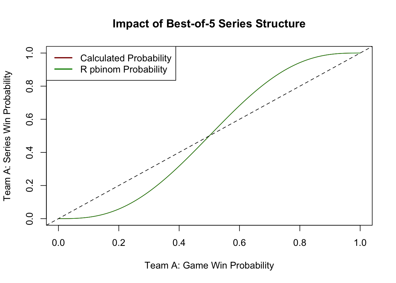
We can plot this against \(p\) to see how the game-win probability impacts the series-win probability \(p\).
p <-seq(0, 1, length.out=101)p_calculated <-6* p^5-15* p^4+10* p^3# pbinom gives probability P(X <= x) or P(X > x) so# to get P(X >= 3), let's just take P(X > 2.9)p_builtin <-pbinom(2.9, 5, p, lower.tail=FALSE)plot(p, p_calculated, type="l", col="red4", xlab="Team A: Game Win Probability", ylab="Team A: Series Win Probability",main="Impact of Best-of-5 Series Structure")lines(p, p_builtin, col="green4")legend("topleft", legend=c("Calculated Probability", "R pbinom Probability"), col=c("red4", "green4"), lwd=2)abline(a=0, b=1, col="black", lty=2)
As we see here, the “best of” structure increases the chance that the “better” team wins the overall series.
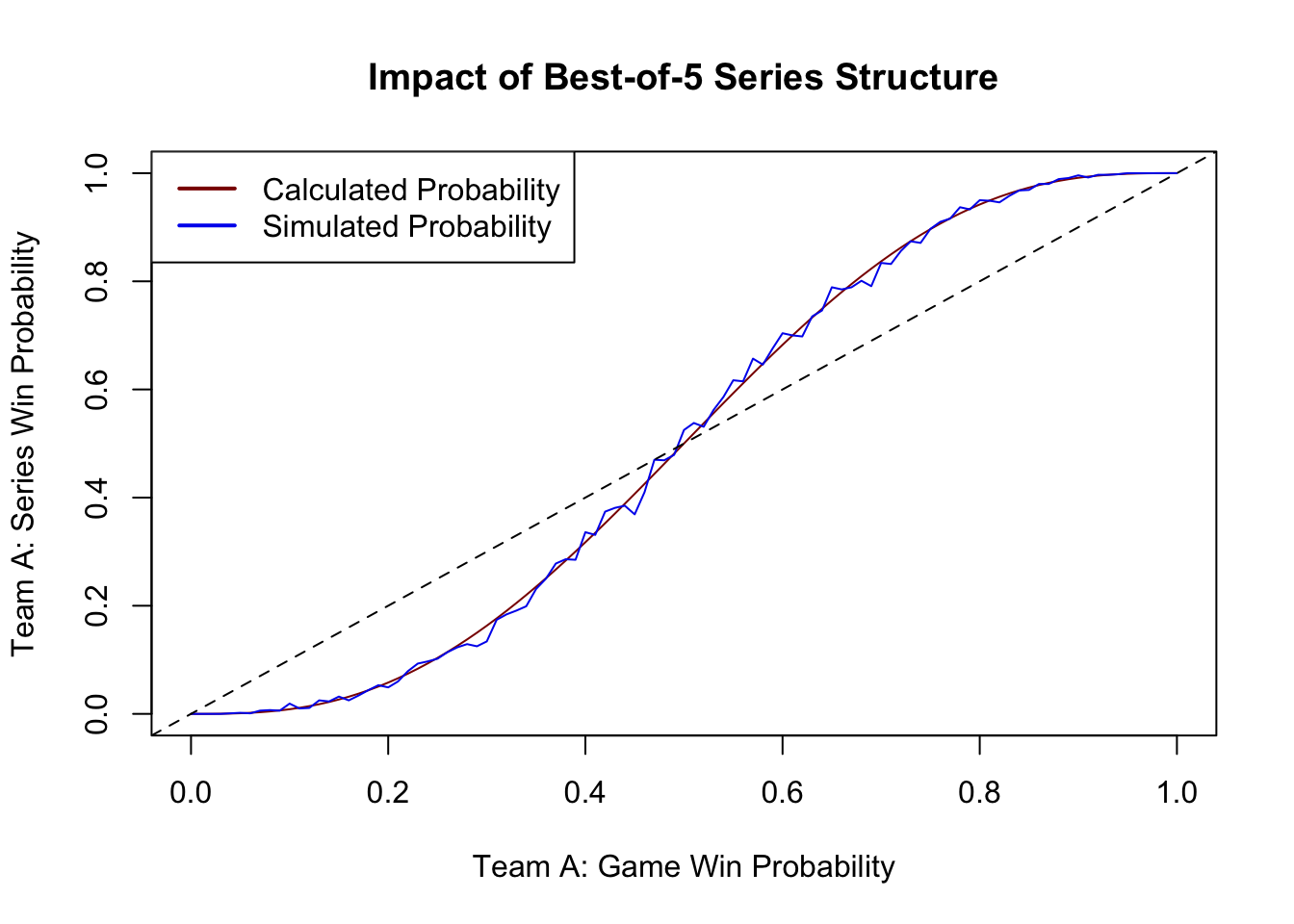
We can also see this empirically in simulation. As always with simulation, we don’t expect exact alignment since simulation still has some randomness and we aren’t doing an infinite number of repetitions.
p <-seq(0, 1, length.out=101)p_calculated <-6* p^5-15* p^4+10* p^3p_empirical <-vapply(p, function(p) mean(rbinom(1000, 5, p) >=3), 0.0)plot(p, p_calculated, type="l", col="red4", xlab="Team A: Game Win Probability", ylab="Team A: Series Win Probability",main="Impact of Best-of-5 Series Structure")lines(p, p_empirical, col="blue2")legend("topleft", legend=c("Calculated Probability", "Simulated Probability"), col=c("red4", "blue2"), lwd=2)abline(a=0, b=1, col="black", lty=2)
Question 2
For a group of 7 people, find the probability that all 4 seasons (winter, spring, summer, fall) occur at least once each among their birthdays, assuming that all seasons are equally likely.
Question History
This is Question BH 1.9.51.
Solution
To compute this probability we use the “naive” (outcome-counting) definition of probability:
\[\P = \frac{\text{\# of outcomes with all four seasons represented}}{\text{\# of total possible outcomes}} \]
The denominator is easy: each person is independent, so there are \(4^7\) possible outcomes.
The numerator is a bit trickier: we have to do some “inclusion-exclusion” math.
Number of “no winter” outcomes: \(3^7\)
Number of “no spring” outcomes: \(3^7\)
Number of “no summer” outcomes: \(3^7\)
Number of “no fall” outcomes: \(3^7\)
Number of “no winter and no spring” outcomes: \(2^7\)
Number of “no winter and no summer” outcomes: \(2^7\)
Number of “no winter and no fall” outcomes: \(2^7\)
Number of “no spring and no summer” outcomes: \(2^7\)
Number of “no spring and no fall” outcomes: \(2^7\)
Number of “no summer and no fall” outcomes: \(2^7\)
Number of “no winter and no spring and no summer” outcomes (all fall): \(1^7\)
Number of “no winter and no spring and no fall” outcomes (all summer): \(1^7\)
Number of “no winter and no summer and no fall” outcomes (all spring): \(1^7\)
Number of “no spring and no summer and no fall” outcomes (all winter): \(1^7\)
The pattern here is actually a bit easier to see if we wrap it up mathematically: if we want to allow \(n\) seasons (of 4), there are \(\binom{4}{n}\)\(n\)-tuples of restrictions. For each of these, we have \(n^7\) possible outcomes, so the total number of outcomes is \[\sum_{n=1}^3 \binom{4}{n}n^7(-1)^(n+1) = 4 * 1^7 - 6 * 2^7 + 4 * 3^7 = 7984\] events that omit at least one season. This gives us a final probability of:
Additionally, we can verify this solution in simulation:
mean(replicate(10000, { # mean(replicate(, INDICATOR)) can be # used to estimate probabilities seasons <-sample(c("Winter", "Spring", "Summer", "Fall"), 7, replace=TRUE)length(unique(seasons)) ==4}))
[1] 0.5133
which is in substantial agreement with our exact result above.
Alternatively, the sample space here is large enough that we can enumerate it in its entirety:
which matches our calculation of the numerator above.
Question 3
Suppose that Ashley is playing a guessing game, where she has a 25% chance of answering a given question correctly (IID). If she answers a question correctly, she gets one point. Let \(Q\) be the total number of questions required for her to get five total points. What is the variance of \(Q\)?
Question History
A version of this question appeared as Question 2 from the Week 4 Quiz. Here, I ask about variance instead of expected value.
Solution
Let \(Q_1\) be the number of attempts Ashley makes to get her first point; \(Q_2\) be the number of additional attempts Ashley makes to get her second point; etc.. Then \(Q = Q_1 + Q_2 + Q_3 + Q_4 + Q_5\).
Each \(Q_i\) is IID Geometric with probability \(p\) and so its variance is given by \(\V[Q_i] = (1-p)/p^2\), as can be seen on the Formula Sheet. Because the \(Q_i\) are IID, their variances add and we obtian \[\V[Q] = \sum_{i=1}^5 \V[Q_i] = \sum_{i=1}^5 \frac{1-p}{p^2} = \frac{5(1-p)}{p^2}\]
At \(p=0.25\), this works out to 60.
If we recognize this as a negative binomial distribution, we can also check it in R directly:
var(rnbinom(100000, 5, 0.25))
[1] 59.84925
Question 4
A group of 50 people are comparing their birthdays; as usual, assume their birthdays are independent, are not February 29, etc. Find the expected number of pairs of people with the same birthday.
Question History
This is the first half of Question BH 4.12.35.
Solution
A given pair of people have a \(1/365\) chance of sharing a birthday. In a group of 50 people, there are \(\binom{50}{2} = 1225\) total pairs. By the properties of indicators and expectations, the expected number of people to share a birthday is simply \(\binom{50}{2} * \frac{1}{365} \approx 3.36\).
We can again verify this experimentally:
mean(replicate(100000, { # mean(replicate(, N)) can be # used to estimate E[N] birthdays <-sample(365, 50, replace=TRUE) N_shares <-sum(outer(birthdays, birthdays, `==`)) (N_shares -50)/2# Remove "self-shares" and divide by 2 (i, j) == (j, i)}))
[1] 3.35946
Question 5
A certain family has 6 children, consisting of 3 boys and 3 girls. Assuming that all birth orders are equally likely, what is the probability that the 3 eldest children are the 3 girls?
Question History
This is Question BH 1.9.24.
Solution
There are \(\binom{6}{3}\) possible orderings (choosing in which of the 6 “slots” to put the 3 girls). Of these, only one has the three girls born first, so the probability is given by:
Suppose \(X \sim \text{Poisson}(\lambda)\), that is \(X\) is a Poisson random variable with mean \(\lambda = \E[X]\). What is the second (non-central) moment of \(X\), i.e., \(\E[X^2]\)?
Question History
This is Question 3 from the Week 4 Quiz.
Solution
We recall that \(\V[X] = \E[X^2] - \E[X]^2\). Rearranging, this gives us \(\E[X^2] = \E[X]^2 + \V[X]\). For a Poisson random variable, we have \(\E[X] = \V[X] = \lambda\), so we obtain:
\[\E[X^2] = \lambda^2 + \lambda.\]
Question 7
Suppose that course grades are distributed as follows:
Grade
A
B
C
D
F
GPA Points
4
3
2
1
0
Fraction of Class
30%
30%
15%
5%
20%
Given that a student did not receive an F, what is the probability they receive an A or a B in the course?
Question History
This is a variant of Question 1 from the Week 4 Quiz. Here, I ask for a conditional probability instead of a conditional expectation.
Solution
To compute the PMF conditional on not failing, we can use the definition of conditional probability
\[\P(A | \text{ not } F) = \frac{\P(A \text{ and not } F)}{\P(\text{not }F)} = \frac{\P(A)}{1 - \P(F)} = \frac{0.3}{1-0.2} = \frac{3}{8}\]
Similarly,
\[\P(B | \text{ not } F) = \frac{\P(B \text{ and not } F)}{\P(\text{not }F)} = \frac{\P(B)}{1 - \P(F)} = \frac{0.3}{1-0.2} = \frac{3}{8}\]
Combining these, we have:
\[\P(A \text{ or } B | \text{ not } F) = \P(A | \text{ not } F) + \P(B | \text{ not } F) = \frac{3}{8} + \frac{3}{8} = \frac{3}{4}\]
Question 8
Suppose that the number of Baruch students to win the lottery each year is Poisson distributed with mean \(2\). What is the probability that an above average (i.e., above mean) number of Baruch students win the lottery next year?
Question History
This is a new question, designed to test your use of PMFs and CDFs.
Solution
We use the complement rule to convert the infinite event “above 2” to a finite set of outcomes “0, 1, or 2”. We then simply use the Poisson PMF: \[\begin{align*}
\P(X > 2) &= 1 - \P(X \leq 2) \\
&= 1 - \sum_{x=0}^2 \P(X = x) \\
&= 1 - \sum_{x=0}^2 \frac{2^x e^{-2}}{x!} \\
&= 1 - \left(\frac{2^0 e^{-2}}{0!}+\frac{2^1 e^{-2}}{1!}+\frac{2^2 e^{-2}}{2!}\right) \\
&= 1 - \left(e^{-2} + 2e^{-2} + 2e^{-2}\right) \\
&= 1 - 5e^{-2} \\
&\approx 32.3\%
\end{align*}\]
We can also compute this more directly in R:
ppois(2, 2, lower.tail=FALSE)
[1] 0.3233236
Here, pDIST(..., lower.tail=FALSE) gives the complimentary CDF.
Question 9
According to the CDC, men who smoke are 23 times more likely to develop lung cancer than men who don’t smoke. Also according to the CDC, 21.6% of men in the US smoke. What is the probability that a man in the US is a smoker, given that he develops lung cancer?
Question History
This is Question BH 2.11.3.
Solution
Let \(C\) be the event that an individual develops lung cancer and let \(S\) be the event that he his a smoker. The CDC data then gives us:
Let \(T\) be the time until a radioactive particle decays and suppose that \(T \sim \text{Exponential}(\lambda)\). The half-life of the particle is the time at which there is a 50% chance that the particle has decayed (i.e., the median of \(T\)). Find the half-life of the particle in terms of \(\lambda\).
To find the median, i.e., the 50% probability point, we first need to compute the CDF. Since \(T\) is exponentially distributed, we can compute its CDF by integrating its PDF:
Suppose the random variables \((X, Y)\) have joint PDF \(f_{(X, Y)}(x, y) = 4xy\) with support on the unit square \([0, 1]^2\). (That is, both \(X\) and \(Y\) can take any value in \([0, 1]\)). What is the conditional expectation of \(X\) given \(Y > 0.5\)
Question History
This is a new question, designed to test your use of conditional PDFs. Due to its use of conditional probabilities and PDFs, this is probably the most advanced question on this test.
Solution
We need to compute the density of \(X\), conditional on \(Y > 0.5\).
It will be useful to first compute the probability that \(Y > 0.5\):
Five students board the Baruch express elevators at the same time from the second floor. Assuming that their destinations are uniformly random (i.e., that they exit at each floor with equal probability), what is the probability that no students exit on the 11th floor? (Recall that the Baruch express elevators stop at the 5th, 8th, and 11th floors.)
Question History
This is Question 1 from the Week 2 Quiz.
Solution
By assumption, each student has a \(2/3\) chance of exiting other than the 11th floor. Because the students are independent, their exit floors are independent events and the associated probabilities may be multiplied: \[\left(\frac{2}{3}\right)^5 \approx 0.13\] Computationally,
Let \[X \sim \mathcal{N}(3, \sqrt{2}^2)\] and \[Y \sim \mathcal{N}(1, \sqrt{2}^2)\] be independent normal random variables. Calculate \(\mathbb{P}(X < Y)\). You may leave your answer in terms of the standard normal CDF \(\Phi(\cdot)\).
Hint: Use the fact that \(Z_1 \sim \mathcal{N}(\mu_1, \sigma_1^2)\) and \(Z_2 \sim \mathcal{N}(\mu_2, \sigma_2^2)\) implies \[aZ_1 + bZ_2 + c \sim \mathcal{N}(a\mu_1 + b\mu_2 + c, a^2\sigma_1^2 + b^2\sigma_2^2)\] for \(Z_1, Z_2\) independent.
Question History
This is a simplified version of Question BH 5.10.25.
Solution
As the hint suggests, let’s look at the distribution of \(X - Y\) since
\[\P(X < Y) = \P(X - Y < 0)\]
Per the hint, \(X - Y\) will have a normal distribution with mean \[\E[X - Y] = \E[X] - \E[Y] = 3 - 1 = 2\] and variance \[\V[X - Y] = \V[X] + \V[Y] = \sqrt{2}^2 + \sqrt{2^2} = 2 + 2 = 4 = 2^2\] so \[X - Y\sim \mathcal{N}(2, 2^2)\]. We then note that \(X - Y = 2 + 2Z\) for standard normal \(Z\), so \[\P(X - Y < 0) = \P(2 + 2Z < 0) = \P(2Z < -2) = \P(Z < -1) = \Phi(-1) \approx 15.8\%.\]
As usual, let’s check this computationally:
X <-rnorm(50000, mean=3, sd=sqrt(2))Y <-rnorm(50000, mean=1, sd=sqrt(2))mean(X < Y)
[1] 0.15714
Question 14
Suppose a random variable \(X\) takes continuous values between 2 and 5. Suppose further that its PDF is \(f_X(x) = c x^2\) for some unknown \(c\). What is \(c\)?
Question History
This is a new question, requiring you to use the fact that PDFs integrate to 1 over their support.
Solution
We know that the PDF must integrate to 1 over the interval \([2, 5]\). Hence: \[\begin{align*}
1 &= \int_2^5 cx^2\,\text{d}x \\
&= \left.\frac{cx^3}{3}\right|_2^5 \\
&= c\left(\frac{5^3}{3} - \frac{2^3}{3}\right) \\
&= 39c \\
\implies c &= \frac{1}{39}
\end{align*}\]
We can, as usual, verify our work computationally:
integrate(function(x) x^2/39, lower=2, upper=5)
1 with absolute error < 1.1e-14
Question 15
In the Gregorian calendar, each year has either 365 days (normal) or 366 (leap year). A year is randomly chosen with probability 3/4 of being a normal year and 1/4 of being a leap year. Find the mean and variance of the number of days in the chosen year.
Question History
This is Question BH 4.12.2.
Solution
Let \(N\) be the number of days in a year. Under the set-up of the problem, it is clear that \(N \sim 365 + \text{Bernoulli}(1/4)\). Hence,
Four players, named A, B, C, and D, are playing a card game. A standard well-shuffled deck of cards is dealt to the players so each player receives a 13 card hand. How many possibilities are there for the hand that play A will get? (Within a hand, the order in which cards were received doesn’t matter.)
Question History
This is Question BH 1.9.12(a).
Solution
Since the order doesn’t matter, we use the binomial coefficient:
For full credit you do not need to compute this exactly.
Question 19
Let \(X\) be the number of Heads in 10 fair coin tosses (IID). Find the conditional variance of \(X\), given that the first two tosses both land Heads.
Question History
This is a slight variation on Question BH 3.12.24(a), asking only for the conditional variance instead of the full conditional PMF.
Solution
Let \(Y = (X - 2) | \{H, H\}\) be the number of Heads in the final 8 coin tosses. Because the tosses are IID Bernoulli(0.5), we can see that \(Y \sim \text{Binomial}(8, 0.5)\). From here, we use the Binomial variance supplied on the Formula Sheet to see that \[\V[Y] = 8 * 0.5 * (1-0.5) = 2.\]
Note that, here, we use the fact that, conditional on some of the Bernoulli trials, a Binomial becomes a smaller Binomial.
Question 20
Suppose that, before a major election, a polling company contacts a large number of likely voters and successfully asks 1000 voters who they intend to vote for. Candidate A’s supporters have a 100% chance of answering the poll if contacted, while Candidate B’s supporters have only a 50% chance of answering the poll. If 75% of respondents say they intend to vote for Candidate A, what is A’s expected fraction of total votes cast on election day?
(You may assume that supporters of candidate A and B are equally likely to vote and that they only differ in their likelihood to respond to the poll. You may also assume only two candidates. You may also assume respondents don’t lie and are otherwise fully representative, except for differential response rates.)
Question History
This is Question 1 from the Week 3 Quiz.
Solution
Let \(A\) be the event that a voter supports candidate A, \(B\) be the event that a voter supports candidate \(B\), and \(R\) be the event that a voter responds to a poll if contacted. We then have:
\[\begin{align*}
\P(R | A) &= 1 \\
\P(R | B) &= 0.5 \\
\P(A | R) &= 0.75
\end{align*}\]
While we could formally use the rules of conditional probability, it is easier to think in “raw counts”. Specifically, if we had 1000 responses, with 75% support for A, that means we had 750 respondents supporting A and 250 supporting B. Since B supporters only have a 50% chance of responding, that implies 500 B supporters total. Hence, the true support rate for candidate A is \(750 / (750 + 500) = 60\%\).