STA 9890 - Supervised Learning: IV. Discriminative Classifiers & Non-Linear Methods

Author

Michael Weylandt

Published

March 18, 2026

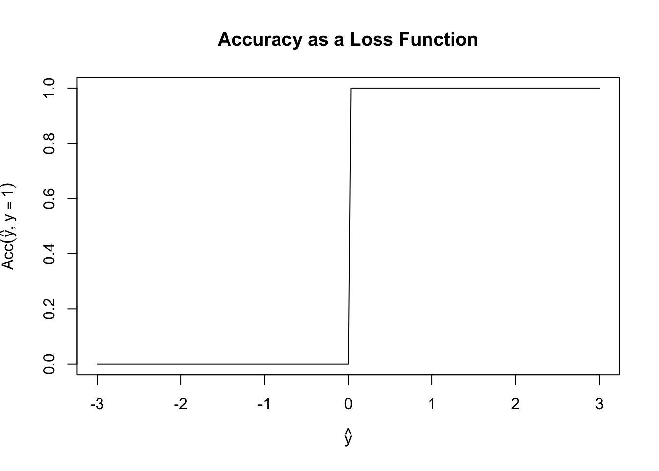
\[\newcommand{\R}{\mathbb{R}} \newcommand{\E}{\mathbb{E}} \newcommand{\V}{\mathbb{V}} \newcommand{\P}{\mathbb{P}} \newcommand{\C}{\mathbb{C}} \newcommand{\K}{\mathbb{K}} \newcommand{\Ycal}{\mathcal{Y}} \newcommand{\Xcal}{\mathcal{X}} \newcommand{\Ccal}{\mathcal{C}} \newcommand{\Hcal}{\mathcal{H}} \newcommand{\Ncal}{\mathcal{N}} \newcommand{\Fcal}{\mathcal{F}} \newcommand{\Ocal}{\mathcal{O}} \newcommand{\Pcal}{\mathcal{P}} \newcommand{\Ucal}{\mathcal{U}} \newcommand{\Dcal}{\mathcal{D}} \newcommand{\bbeta}{\mathbf{\beta}} \newcommand{\bone}{\mathbf{1}} \newcommand{\bzero}{\mathbf{0}} \newcommand{\ba}{\mathbf{a}} \newcommand{\bb}{\mathbf{b}} \newcommand{\bc}{\mathbf{c}} \newcommand{\bu}{\mathbf{u}} \newcommand{\bv}{\mathbf{v}} \newcommand{\bw}{\mathbf{w}} \newcommand{\bx}{\mathbf{x}} \newcommand{\by}{\mathbf{y}} \newcommand{\bz}{\mathbf{z}} \newcommand{\bf}{\mathbf{f}} \newcommand{\bX}{\mathbf{X}} \newcommand{\bA}{\mathbf{A}} \newcommand{\bB}{\mathbf{B}} \newcommand{\bC}{\mathbf{C}} \newcommand{\bD}{\mathbf{D}} \newcommand{\bU}{\mathbf{U}} \newcommand{\bV}{\mathbf{V}} \newcommand{\bI}{\mathbf{I}} \newcommand{\bH}{\mathbf{H}} \newcommand{\bW}{\mathbf{W}} \newcommand{\bY}{\mathbf{Y}} \newcommand{\bK}{\mathbf{K}} \newcommand{\argmin}{\text{arg\,min}} \newcommand{\argmax}{\text{arg\,max}} \newcommand{\MSE}{\text{MSE}} \newcommand{\Tr}{\text{Tr}}\]

Discriminative Classifiers

This week we begin to examine discriminative classifiers. Unlike generative classifiers, which attempt to model \(\bx\) as a function of \(y\) and then use Bayes’ rule to invert that model, discriminative classifiers take the more standard approach of directly modeling \(y\) as a function of \(\bx\). This is the approach you have already seen in our various variants of OLS.

Why Not Accuracy Maximization?

As we saw in our regression unit, we can pose many interesting estimators as loss minimization problems. For least squares, we primarily focused on mean squared error (MSE) as a loss function, though we also briefly touched on MAE, MAPE, and ‘check’ losses. There is not a single ‘canonical’ loss for the classification setting and different choices of loss will yield different classifiers.

Before we build our actual first loss, it is worth asking why we can’t use something like classification accuracy as our loss function. Specifically, define \[\text{Acc}(y, \hat{y}) = \begin{cases} 1 & y = \text{sign}(\hat{y}) \\ 0 & y \neq \text{sign}(\hat{y}) \end{cases}\] Here we consider the case where \(\hat{y}\) may be real-valued as a (slight) generalization of probabilistic classification and we use the \(\pm 1\) convention for the two classes.

Fixing \(y = 1\), \(\text{Acc}\) has the following shape:

y_hat <- seq(-3, 3, length.out=201)
acc <- function(y_hat, y=1) sign(y_hat) == sign(y)

plot(y_hat, acc(y_hat), type="l",
     xlab=expression(hat(y)),
     ylab=expression(Acc(hat(y), y==1)), 
     main="Accuracy as a Loss Function")

This is a terrible loss function! It is both non-convex (can you see why?) and just generally unhelpful. Because it is flat almost everywhere, we have no access to gradient information (useful for fitting) or to any sense of ‘sensitivity’ to our loss. In this scenario, if \(y=1\), both \(\hat{y}=0.00001\) and \(\hat{y}=0.9999\) have the same accuracy even though the latter is a more ‘confident’ prediction.

OLS for Classification?

So if not accuracy, where else might we get a good loss function? You might first ask if we an use OLS? It works perfectly well for regression and we know it is well-behaved, so what happens if we try it for classification? The answer is … complicated.

OLS as a loss function for classification is a bit strange, but it turns out to be more-or-less fine. In particular, OLS can be used to evaluate probabilistic classifiers, where it is known as the Brier score. OLS as a predictor can be a bit more problematic: in particular, if we just predict with \(\P(y=1) = \bx^{\top}\bbeta\), we have to deal with the fact that \(\hat{y}\) can be far outside a \([0, 1]\) range we might want from a probabilistic classifier. In certain limited circumstances, we can assume away this problem (perhaps by putting specific bounds on \(\bx\)), but these fixes are fragile. Alternatively, we can try to ‘patch’ this approach and use a classifier like

\[\P(y=1) = \begin{cases} 1 & \bx^{\top}\bbeta > 1 \\ 0 & \bx^{\top}\bbeta < 0 \\ \bx^{\top}{\bbeta} & \text{ otherwise}\end{cases}\]

Even if this feels a bit unsophisticated, ii is not awful, but it still struggles from the ‘long flat region’ problems that accuracy encounters.

At this point, it’s hopefully clear that it will be a bit hard to ‘hack together’ a suitable loss and that we might benefit from approaching the problem with more theoretical grounding.

Deriving Logistic Regression

While we argued that OLS is well-grounded in MSE alone, we can recall it has additional connections to the Gaussian. These “Gaussian vibes” were not essential to making OLS work, but they were useful in deriving OLS as a sensible procedure. Can we do something similar for classification? That is, can we assume a ‘working model’ to come up with a good loss function and then use it, even if we doubt that the model is ‘correct’?

As with all leading questions, the answer is of course a resounding yes. We start from the rather banal observation that \(y\) must have a Bernoulli distribution conditional on \(\bx\). After all, the Bernoulli is (essentially) the only \(\{0, 1\}\) distribution we have to work with. So we really just need a way to model the \(p\) parameter of a Bernoulli as a function of \(\bx\). Because we love linear models, we may choose to set \(p = \bx^{\top}\bbeta\), but this gets us back to the range problem we had above.

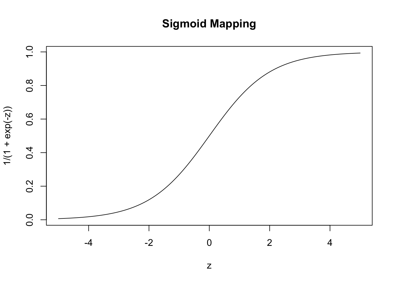
Specifically, we require the Bernoulli parameter to take values in \([0, 1]\) but our linear predictor \(\bx^{\top}\bbeta\) takes values in all of \(\R\). We can fix this with a simple ‘hack’: we need a function that ‘connects’ \(\R\) to \([0, 1]\). If we call this function \(\mu\), we then can specify our whole model as \[y | \bx \sim \text{Bernoulli}(\mu(\bx^{\top}\bbeta))\] and reduce our problem to estimating \(\bbeta\). Where can we get such a function?

The most common choice is \[\mu(z) = \frac{e^z}{1+e^z} = \frac{1}{1+e^{-z}}\], which is known as the logistic or sigmoid function due to its ‘s-like’ shape:

z <- seq(-5, 5, length.out=201)
plot(z, 1/(1+exp(-z)), type="l", main="Sigmoid Mapping")

More generally, we can use essentially the CDF of any random variable supported on the real line as a choice of \(\mu\): since CDFs map the support onto the \([0, 1]\) range they are perfect for this choice. Unfortunately, most CDFs are a bit unwieldy so this approach, while theoretically satisfying, is not too widely used in practice. If you see it, the most common choice is \(\mu(z) = \Phi(z)\), the normal CDF, resulting in a method known as “probit” regression (after ‘probability integral transform,’ an old-fashioned name for the CDF) or \[\mu(z) = \frac{\tan^{-1}(z)}{\pi} + \frac{1}{2}\] which gives a method known as “cauchit” regression, since this is the CDF of the standard Cauchy distribution. These choices are far less common than the default sigmoid we used above. Generally, they are only slightly different in practice and far more computationally burdensome and just aren’t really worth it.

Returning to our default sigmoid, we now have the model \[ y | \bx \sim \text{Bernoulli}\left(\frac{1}{1+e^{-\bx^{\top}\bbeta}}\right)\] This model is well-posed (in the sense that the distribution ‘fits’ the data and we are guaranteed never to put invalid parameters in) but we don’t yet have a way to use it as a loss function.

From Model to Loss Function

We can build a loss-function by relying on the maximum likelihood principle. The maximum likelihood principle is a core idea of statistics - and one you will explore in much greater detail in other courses - but, in essence, it posits that we should use the (negative) PMF or PDF as our loss function. Specifically, the ML principle says that, if many models could fit our data, we should pick the one that makes our data most probable (as determined by the PMF/PDF).

Before we work out the ML estimator (MLE) for our classification model, let’s take a brief detour and look at the MLE for (Gaussian) regression. Specifically, if we assume a model \[y \sim \Ncal(\bx^{\top}\bbeta, \sigma^2)\] for known \[\sigma^2\], the PDF of the training point \((\bx_1, y_1)\) is

\[p(y_1 | \bx_1) = \frac{1}{\sqrt{2\pi\sigma^2}}\exp\left\{-\frac{\|y_1 - \bx_1^{\top}\bbeta\|_2^2}{2\sigma^2}\right\}\]

If we have a set of \(n\) IID training data points, the joint PDF can be obtained by multiplying together PDFs (IID is great!) to get

\[\begin{align*} p(\Dcal_{\text{train}}) &= \prod_{i=1}^n p(y_i | \bx_i) \\ &= \prod_{i=1}^n \frac{1}{\sqrt{2\pi\sigma^2}}\exp\left\{-\frac{\|y_i - \bx_i^{\top}\bbeta\|_2^2}{2\sigma^2}\right\} \\ &= (2\pi\sigma^2)^{-n/2}\exp\left\{-\frac{1}{2\sigma^2}\sum_{i=1}^n \|y_i - \bx_i^{\top}\bbeta\|_2^2\right\} \\ &= (2\pi\sigma^2)^{-n/2}\exp\left\{-\frac{1}{2\sigma^2} \|\by - \bX\bbeta\|_2^2\right\} \\ \end{align*}\]

We could maximize this, but a few minor tweaks make the problem much easier:

Since all of the action is in an exponential, we might as well maximize the log of the PDF instead of the raw PDF. Since logarithms are a monotonic transformation, this won’t change our minimizer. Similarly, we will also strategically drop some constant terms as they also do not change the minimizer.
By convention, we like to minimize more than maximize, specifically when dealing with convex approaches, so we will introduce a sign flip.

\[\begin{align*} \hat{\bbeta} &= \argmax_{\bbeta} p(\Dcal_{\text{train}}) \\ &= \argmax_{\bbeta} \log p(\Dcal_{\text{train}}) \\ &= \argmax_{\bbeta} \log\left( (2\pi\sigma^2)^{-n/2}\exp\left\{-\frac{1}{2\sigma^2}\sum_{i=1}^n \|\by - \bX\bbeta\|_2^2\right\}\right) \\ &= \argmax_{\bbeta} -\frac{n}{2}\log(2\pi\sigma^2) -\frac{1}{2\sigma^2} \|\by - \bX\bbeta\|_2^2 \\ &= \argmin_{\bbeta} \frac{n}{2}\log(2\pi\sigma^2) + \frac{1}{2\sigma^2} \|\by - \bX\bbeta\|_2^2 \\ &= \argmin_{\bbeta} \frac{1}{2}\|\by - \bX\bbeta\|_2^2 \end{align*}\]

Why were we able to do the simplifications in the last line? (You might also recognize the penultimate line as a term used in the AIC of a linear model.)

This is quite cool! If we assume \(\by\) follows a particular Gaussian, we get OLS by applying the general MLE approach. Deeper statistical theory tells us that the MLE is (essentially) optimal, so if our data is not too ‘un-Gaussian’ it makes sense that the Gaussian MLE (OLS) will perform reasonably well. Since many things in this world are Gaussian-ish, OLS is optimal-ish for a large class of interesting problems.

Returning to our classification problem, we see that if our training data is IID, the MLE can be obtained by minimizing the negative sum of the log PDFs. For space, we often start from this point instead of doing the full set of manipulations from scratch.

So what is the Bernoulli log PMF? Recall that if \(B \sim \text{Bernoulli}(p)\), its PMF is given by:

\[\P(B=k) = \begin{cases} p & k=1 \\ 1-p & k = 0 \end{cases}\]

or more compactly,

\[\P(B = k) = p^k(1-p)^(1-k)\]

Taking logarithms, we have

\[\log \P(B = k) = k \log p + (1-k) \log(1-p)\]

and hence the negative log-likelihood:

\[-\log \P(B = k) = -k \log p -(1-k) \log(1-p)\]

From our working model, we take \(p = 1/(1+e^{-\bx^{\top}\bbeta})\) so our joint MLE is given by:

\[\hat{\bbeta} = \argmin_{\bbeta} \sum_{i=1}^n -y_i \log\left(1/(1+e^{-\bx_i^{\top}\bbeta})\right) - (1-y_i)\log\left(1 - 1/(1+e^{-\bx_i^{\top}\bbeta})\right)\]

This is still quite hairy, so let’s simplify it. In the first term, we note that \(-\log(1/x) = \log x\) to get:

\[\hat{\bbeta} = \argmin_{\bbeta} \sum_{i=1}^n y_i \log\left(1+e^{-\bx_i^{\top}\bbeta}\right) - (1-y_i)\log\left(1 - 1/(1+e^{-\bx_i^{\top}\bbeta})\right)\]

For the second term, note that

\[1-\frac{1}{1+e^{-z}} = \frac{1+e^{-z} - 1}{1+e^{-z}} = \frac{e^{-z}}{1+e^{-z}} \implies \log\left(1-\frac{1}{1+e^{-z}}\right) = -z - \log(1 + e^{-z})\]

so we get:

\[\begin{align*} \hat{\bbeta} &= \argmin_{\bbeta} \sum_{i=1}^n y_i \log\left(1+e^{-\bx_i^{\top}\bbeta}\right) - (1-y_i)\log\left(1 - 1/(1+e^{-\bx_i^{\top}\bbeta})\right) \\ &= \argmin_{\bbeta} \sum_{i=1}^n y_i \log\left(1+e^{-\bx_i^{\top}\bbeta}\right) - (1-y_i)\left[-\bx_i^{\top}\bbeta + \log\left(1+e^{-\bx_i^{\top}\bbeta}\right)\right] \\ &= \argmin_{\bbeta} \sum_{i=1}^n y_i \log\left(1+e^{-\bx_i^{\top}\bbeta}\right) + (1-y_i)\left[\bx_i^{\top}\bbeta + \log\left(1+e^{-\bx_i^{\top}\bbeta}\right)\right] \\ &= \argmin_{\bbeta} \sum_{i=1}^n y_i \log\left(1+e^{-\bx_i^{\top}\bbeta}\right) + \left[\bx_i^{\top}\bbeta + \log\left(1+e^{-\bx_i^{\top}\bbeta}\right)\right] -y_i\left[\bx_i^{\top}\bbeta + \log\left(1+e^{-\bx_i^{\top}\bbeta}\right)\right]\\ &= \argmin_{\bbeta} \sum_{i=1}^n-y_i \bx_i^{\top}\bbeta + \bx_i^{\top}\bbeta + \log\left(1-e^{-\bx_i^{\top}\bbeta}\right) \end{align*}\]

We could work in this form, but it turns out to actually be a bit nicer to ‘invert’ some of the work we did above to get rid of a term. In particular, note

\[z + \log(1-e^{-z}) = \log(e^z) + \log(1-e^{-z}) = \log(e^z + e^{z-z}) = \log(1 + e^z)\]

which gives us:

\[\hat{\bbeta} = \argmin_{\bbeta} \sum_{i=1}^n-y_i \bx_i^{\top}\bbeta + \log\left(1+e^{\bx_i^{\top}\bbeta}\right)\]

Wow! Long derivation. And we still can’t actually solve this!

Unlike OLS, where we could obtain a closed-form solution, we have to use an iterative algorithm here. While we could use gradient descent, we can get to an answer far more rapidly if we use more advanced approaches. Since this is not an optimization course, we’ll instead use some software to solve for us:

# Generate data from the logistic model
n <- 500
p <- 5
X    <- matrix(rnorm(n * p), ncol=p)
beta <- c(1, 2, 3, 0, 0)

P <- 1/(1+exp(-X %*% beta))
y <- rbinom(n, size=1, prob=P)

# Use optimization software
# See https://cvxr.rbind.io/cvxr_examples/cvxr_logistic-regression/ for details
library(CVXR)


Attaching package: 'CVXR'

The following object is masked from 'package:purrr':

    is_vector

The following object is masked from 'package:stats':

    power

beta <- Variable(p)
eta  <- X %*% beta

objective <- sum(- y * eta + logistic(eta))
problem   <- Problem(Minimize(objective))

beta_hat <- solve(problem)$getValue(beta)

beta_hat
1.0325356
2.1793484
3.0161457
-0.0857759
-0.2758691

Not too bad, if we compare this to R’s built-in logistic regression function, we see our results basically match:

summary(glm(y ~ X + 0, family=binomial))


Call:
glm(formula = y ~ X + 0, family = binomial)

Coefficients:
   Estimate Std. Error z value Pr(>|z|)    
X1  1.03254    0.16129   6.402 1.54e-10 ***
X2  2.17935    0.23030   9.463  < 2e-16 ***
X3  3.01615    0.29303  10.293  < 2e-16 ***
X4 -0.08578    0.15175  -0.565   0.5719    
X5 -0.27587    0.14054  -1.963   0.0497 *  
---
Signif. codes:  0 '***' 0.001 '**' 0.01 '*' 0.05 '.' 0.1 ' ' 1

(Dispersion parameter for binomial family taken to be 1)

    Null deviance: 693.15  on 500  degrees of freedom
Residual deviance: 294.76  on 495  degrees of freedom
AIC: 304.76

Number of Fisher Scoring iterations: 6

Good match!

Note that, in the above, we had to use the logistic function built into CVX. If we used log(1+exp(eta)), the solver would not be able to prove that it is convex and would refuse to try to solve. See the CVX documentation for more details.

We can compute accuracy after defining a ‘decision rule’. Here, let’s just round the predicted probability

p_hat <- 1/(1 + exp(-X %*% beta_hat))
y_hat <- round(p_hat)

mean(y_hat == y)

[1] 0.884

Now that we have this toolkit built up, we can also easily apply ridge and lasso penalization:

penalty <- sum(abs(beta))

lasso_problem <- Problem(Minimize(objective + 9 * penalty))
beta_hat_lasso <- solve(lasso_problem)$getValue(beta)

0.6505892
1.4994013
2.0969206
0.0000000
-0.0727027

We got some sparsity, as we would expect with \(\ell_1\) penalization.

Generalized Linear Models

The approach we took here is a special case of a generalized linear model: generalized linear models (GLMs) consist of three parts:

A linear model for the ‘core predictor’ \(\eta = \bX\bbeta\);
A sampling distribution for the data \(y \sim \text{Dist}\); and
An ‘adaptor’ function¹, \(\mu\), that maps \(\eta \in \R\) to the parameter space of \(y\): specifically, we need \(\E[y | \bx] = \mu(\bx^{\top}\bbeta)\).

The adaptor function needs to be smooth (for nice optimization properties) and monotonic (or else the interpretation gets too weird), but we otherwise have some flexibility. As noted above, if we pick \(\mu\) to be the normal or Cauchy CDFs, we get alternative ‘Bernoulli Regressions’ (probit and cauchit).

We can generalize the model for \(\eta\) by allowing it to be an additive (spline) model or a kernel method. To fit splines, you can use the gam function from the mgcv function.

Finally, we also have choices in the sampling distribution. While normal and Bernoulli are the most common, you will also sometimes see Poisson and Gamma in the wild. For both of these, the mean is a positive value, so we require an adaptor that maps \(\R\) to \(\R \geq 0\) and we typically take \(\mu(z) = e^z\).

A good exercise is to repeat the above analysis for Poisson regression and compare your result (obtained with CVXR) to the Poisson regression built into R.

Loss Functions for Classification

We now have a workable loss function for discriminative classification. Returning to our example from above (changed to \(\{0, 1\}\) convention briefly). Let us set \(\alpha = y\hat{y}\) and investigate our loss functions as a property of \(\alpha\):

alpha <- seq(-3, 3, length.out=201)
acc     <- function(alpha) ifelse(alpha < 0, 1, 0)
lr_loss <- function(alpha) log(1 + exp(-2*alpha))

plot(alpha, acc(alpha), type="l",
     xlab=expression(alpha),
     ylab="Loss", 
     main="Classification Losses", 
     ylim=c(0, 5))
lines(alpha, lr_loss(alpha), col="red4")
legend("topright", 
       col=c("black", "red4"), 
       lwd=2, 
       legend=c("Accuracy", "Logistic Regression"))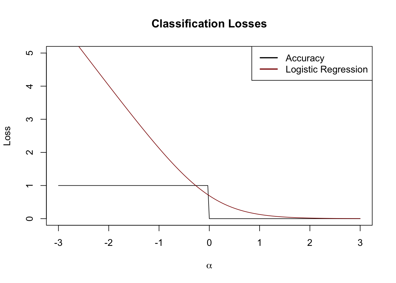

We see here that the logistic loss defines a convex surrogate of the underlying accuracy. Just like we used \(\ell_1\) as a tractable approximation for best squares, logistic regression can be considered a tractable approximation for accuracy minimization.²

Other useful loss functions can be created using this perspective, perhaps none less important than the hinge loss, which gives rise to a classifier known as the support vector machine (SVM).

Support Vector Machines

In this section, we go back to \(\{\pm 1\}\) convention.

Instead of using a logistic loss, consider a hinge loss of the form

\[H(y, \hat{y}) = (1 - y\hat{y})_+\]

When \(y = \hat{y}=1\) or \(y = \hat{y} = 0\), this is clearly 0 as we would expect from a good loss. What happens for cases where our prediction is wrong or not ‘full force’, say \(\hat{y} = 1/2\).

Looking ahead, we will use a linear combination of features to create \(\hat{y} = \bx^{\top}\bbeta\) yielding:

\[H(\bbeta) = (1 - y \bx^{\top}\bbeta)_+\]

If \(y=1\), we get zero loss so long as \(\bx^{\top}\bbeta > 1\) and a small loss for \(0 < \bx^{\top}\bbeta < 1\). As \(\bx^{\top}\bbeta\) crosses zero and goes negative, the loss grows linearly without bound. (Reverse all of this for the case \(y = -1\).) This is an interesting loss function: we cannot make our loss decrease as our predictions become ‘more right’, but our loss continues to increase as our prediction becomes ‘more wrong’.

Visually, we can draw this on our plot from above:

alpha <- seq(-3, 3, length.out=201)
acc     <- function(alpha) ifelse(alpha < 0, 1, 0)
lr_loss <- function(alpha) log(1 + exp(-2*alpha))
hinge_loss <- function(alpha) pmax(0, 1-alpha)

plot(alpha, acc(alpha), type="l",
     xlab=expression(alpha),
     ylab="Loss", 
     main="Classification Losses", 
     ylim=c(0, 5))
lines(alpha, lr_loss(alpha), col="red4")
lines(alpha, hinge_loss(alpha), col="green4")
legend("topright", 
       col=c("black", "red4", "green4"), 
       lwd=2, 
       legend=c("Accuracy", "Logistic Regression", "Hinge Loss"))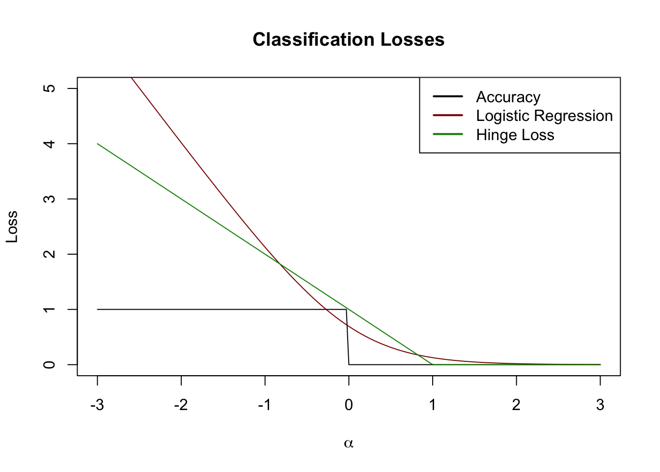

This is also a pretty nice surrogate loss. In this case, let’s just go ‘straight at it’ to construct a classifier:

\[\hat{\bbeta} = \argmin \sum_{i=1}^n (1-y_i \bx_i^{\top}\bbeta)_+\]

This classifier is not uniquely defined for many problems (because of the long flat part of the loss), so it is conventional to add a regularization term to the SVM:

\[\hat{\bbeta} = \argmin \sum_{i=1}^n (1-y_i \bx_i^{\top}\bbeta)_+ + \lambda \|\bbeta\|_2^2\]

We can solve this directly using CVX as follows:

# Generate data from the logistic model and fit an SVM
n <- 500
p <- 5
X    <- matrix(rnorm(n * p), ncol=p)
beta <- c(1, 2, 3, 0, 0)

P <- 1/(1+exp(-X %*% beta))
y <- rbinom(n, size=1, prob=P)
## Convert to +/-1 convention
y <- 2 * y - 1

library(CVXR)

beta <- Variable(p)
eta  <- X %*% beta

objective <- sum(pos(1 - y * eta)) + 0.5 * norm2(beta)^2
problem   <- Problem(Minimize(objective))

beta_hat <- solve(problem)$getValue(beta)

Using the decision rule \(\hat{y} = \text{sign}(\bx^{\top}\bbeta)\), this gives us good accuracy:

mean(sign(X %*% beta_hat) == y)

[1] 0.848

This is comparable to what we got for logistic regression even though:

the loss function is ‘wrong’ (doesn’t model the DGP)
we did no tuning of the ridge parameter

So, all in all, pretty impressive.

SVMs are a remarkably powerful and general classification technology. Before we move past them, we will now take a second perspective focusing on the geometry of SVMs.

SVM: The Geometric Viewpoint

Non-Linear Methods

We have now developed a variety of tools for linear regression and for linear classification. These work well - particularly in low SNR (high dimension / low sample size) scenarios - but they have a necessarily limited capacity. When we have lots of training data, how can we go further? By using non-linear methods of course!

In this section we introduce several methods for non-linear regression. These techniques can all be easily adapted to classification, but we’ll develop them for regression as the math is a bit simpler. We also pause to consider when non-linear methods can actually be expected to outperform linear methods.

Also note that we are arguably being a bit ‘sloppy’ about what we mean by ‘linear’ methods. For purposes of these notes, we define a ‘linear’ method as one where the fitted model has a linear response to changes in the inputs; formally, one where

\[\frac{\partial y}{\partial x_i} = \beta_i \text{ (a constant) for all } i \in \{1, \dots, p\}\]

This definition includes things like best-subsets and lasso regression, which are not linear functions of \(\by\), but excludes things like polynomial regression.³ In the above definition, each \(\beta_i\) is essentially a regression coefficient, and values of \(i\) where \(\beta_i = 0\) are non-selected variables if we are using a sparse method.

Non-Linearity via Linear Combination of Non-Linear Parts

We have spent the previous few weeks developing a set of tools for building linear models of \(\by\). Specifically, we have sought ways to approximate \(\E[y | \bx]\) as a weighted sum of each \(x_i\):

\[ \E[y | \bx] \approx \langle \bx, \hat{\bbeta} \rangle = \sum_{i=1}^p x_i \hat{\beta}_i\]

For situations where the relationship is nearly (or even truly) linear, this approximation can be quite useful and good estimates of the \(\beta_i\) coefficients can lead to accurate estimates of \(\E[y | \bx]\), and ultimately accurate prediction of test set response \(\by\). Using the bias-variance decomposition, we have seen that it is often worthwhile to accept a bit of bias in estimation of each \(\beta_i\) if it is compensated by a worthwhile reduction in the variance of \(\beta_i\).

We can further refine this equality by decomposing bias a bit further:

\[\MSE = \text{Irreducible Error} + \text{Variance} + \text{Model Bias}^2 + \text{Estimation Bias}^2\]

Here, we have decomposed \(\text{Bias}^2\) into two terms:

\(\text{Model Bias}^2\): a measure of the systematic error arising from use of a linear model to predict a non-linear DGP
\(\text{Estimation Bias}^2\): a measure of the systematic error arising from use of a regularized estimation procedure which exhibits shrinkage

Put another way, “Model Bias” results from use of a linear model when something non-linear should be used, while “Estimation Bias” arises from the use of a biased method (like ridge regression) instead of something nominally unbiased like OLS. For the previous two weeks, we have mainly focused on linear models for linear DGPs, so model bias has been zero. If we expand our gaze to non-linear DGPs, we have to deal with model bias a bit more directly. As with estimation bias, it is frequently worthwhile to accept model bias to reduce variance; see more discussion below.

Polynomial Expansion

You have likely already seen polynomial expansion (or polynomial regression) in previous courses. Essentially, PE fits a low(-ish)-order polynomial instead of a line to data. More formally, let \(f(\bx) \equiv \E[y|\bx]\) be the regression function (best possible predictor) that week seek to approximate from noisy observations. Standard linear regression essentially seeks to fit a first-order Taylor approximation of \(f\) around some point \(\overline{\bx}\):

\[\begin{align*} f(\bx) &\approx f(\overline{\bx}) + \nabla_f(\bx_0)^{\top}(\bx - \overline{\bx}) \\ &= f(\overline{\bx}) + \sum_{i=1}^p \left. \frac{\partial f}{\partial x_i}\right|_{x = \overline{x}_i}(x_i - \overline{x}_i) \end{align*}\]

If we rearrange this a bit, we get

\[\begin{align*} f(\bx) &\approx f(\overline{\bx}) + \sum_{i=1}^p \left. \frac{\partial f}{\partial x_i}\right|_{x = \overline{x}_i}(x_i - \overline{x}_i) \\ &= \underbrace{\left(f(\overline{\bx}) - \sum_{i=1}^p \left.\frac{\partial f}{\partial x_i}\right|_{x_i=\overline{x}_i}\overline{x}_i\right)}_{=\beta_0} + \sum_{i=1}^p \underbrace{\left.\frac{\partial f}{\partial x_i}\right|_{x_i=\overline{x}_i}}_{=\beta_i} x_i\\ &= \beta_0 + \sum_{i=1}^p x_i \beta_i \end{align*}\]

so we see that the regression coefficients are more-or-less the (suitably-averaged) partial derivatives of \(f\) while the intercept is the value of \(f\) at the center of our expansion (\(f(\overline{\bx})\)) plus some differential adjustments. Note that, if the variables \(\bX\) are centered so that \(\E[\bX] = \bzero\), the intercept is exactly the average value of \(f\), as we would expect.

Clearly, this linear approximation will do better in the situations where Taylor expansions generally perform better: when i) the derivative of \(f\) is roughly constant and ii) the higher order terms are small. This makes sense: if \(f\) is very-close-to-linear, there is minimal loss from fitting a linear approximation to \(f\); if \(f\) is very non-linear, however, a linear approximation can only be be so good, and we are saddled with significant model bias.

If we want to mitigate some of that model bias, we can choose to use a higher-order Taylor series. If we examine a second order Taylor series, we get a similar approximation as before, where \(\Hcal\) denotes the Hessian matrix of second derivatives:

\[\begin{align*} f(\bx) &\approx f(\overline{\bx}) + \nabla_f(\bx_0)^{\top}(\bx - \overline{\bx}) + \frac{1}{2}(\bx - \overline{\bx})^{\top}\Hcal_f(\overline{\bx})(\bx - \overline{\bx})^{\top} \end{align*}\]

After some rearrangement this becomes:

\[f(\bx) \approx \beta_0 + \sum_{i=1}^p \frac{\partial f}{\partial x_i} x_i +\sum_{i=1}^p \frac{\partial^2 f}{\partial x_i^2} x_i^2 + \sum_{\substack{i, j = 1 \\i \neq j}}^p \frac{\partial^2 f}{\partial x_i \partial x_j} x_ix_j\]

We recognize the constant term (intercept) and first order terms (linear slopes) from before, but now we have added two types:

Second order terms (\(x_i^2\)): these capture higher order non-linearities in a single variable. For example, if \(y = x^2\), then the ‘true fit’ really lies in the second order term \(\partial^2f / \partial x^2 = 2\) instead of any linear approximation
Cross terms (\(x_ix_j\)): these capture non-linear (non-additive) multi-variate relationships between features. You may have seen these before as interaction terms.

Rules of thumb vary as to which set of terms are more important. Historically, statisticians have tended to put in the interaction (cross) terms first, though this is far from universal practice. In particular, when dealing with ‘binary’ variables, the higher order term is unhelpful: if a feature is \(0/1\) (did the patient receive the drug or not?), adding a squared term has no effect since \(0^2 = 0\) and \(1^2 = 1\).

Regardless, this is why we sometimes use ‘polynomial expansion’ of our original variables. We are trying to capture the higher-order (non-linear) terms of the Taylor approximation.

It is worth thinking about what happens when we add higher-order terms to our model. In particular, note that we i) pick up some correlation among features; and ii) we will generally have more variance since we have more features. In practice, the correlation isn’t too much of a problem and the actual polynomials fit by, e.g., poly in R are modified to remove correlation. The variance however can be a more significant problem.

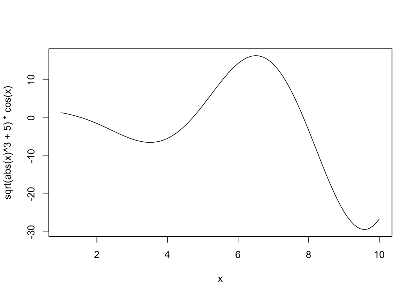
Let’s see this in action. Let’s first consider fitting polynomial regression to a simple (univariate) non-linear function: \(f(x) = \sqrt{|x|^3 + 5} * \cos(x)\)

curve(sqrt(abs(x)^3 + 5) * cos(x), from=1, to=10)

This is not too non-linear. It’s still very smooth (analytic in the jargon) and should be relatively easy to fit. Let’s also generate some noisy observations of this function.

n <- 25
# Linear regression doesn't care about the order of our data, but plotting does
# so sorting gives better visuals
x <- sort(runif(n, 2, 10)) 
Ey <- sqrt(abs(x)^3 + 5) * cos(x)
y <- Ey + rnorm(n, sd=3)


x_grid <- seq(min(x), max(x), length.out=501)
Ey_grid <- sqrt(abs(x_grid)^3 + 5) * cos(x_grid)

plot(x, y)
lines(x_grid, Ey_grid)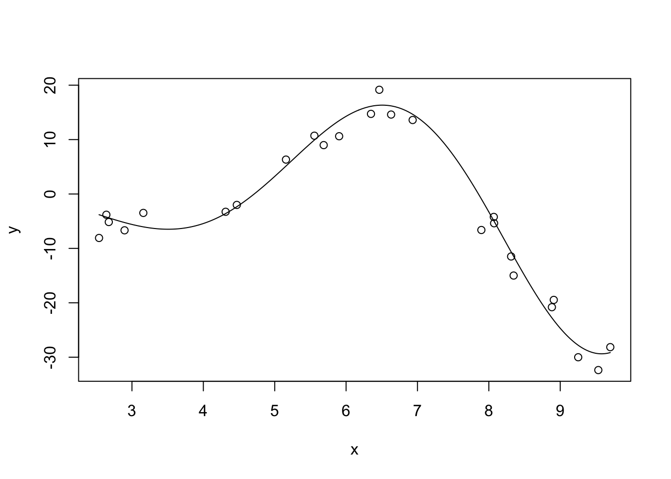

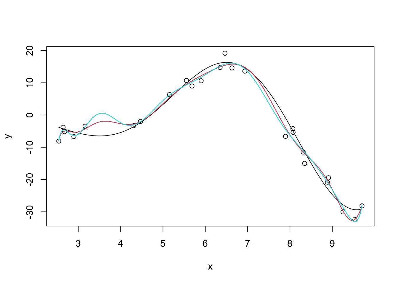
We can now fit some linear models to this data (shown in color): we use R’s built-in poly function to automatically create the polynomials we seek. You can think of poly(x, k) as creating k features \(x^1, x^2, \dots, x^k\) but it actually does something a bit more subtle under the hood to make model fitting a bit more numerically stable.

plot(x, y)
lines(x_grid, Ey_grid)

for(k in 1:5){
    m <- lm(y ~ poly(x, k))
    
    yhat <- predict(m, data.frame(x = x_grid))
    lines(x_grid, yhat, col=k+1)
}

legend("bottomleft",
    c("True Regression Function", 
         "First Order (Linear) Fit",
         "Second Order (Quadratic) Fit", 
         "Third Order (Cubic) Fit", 
         "Fourth Order (Quartic) Fit",
         "Fifth Order (Quintic) Fit"), 
       col=1:6, lty=1)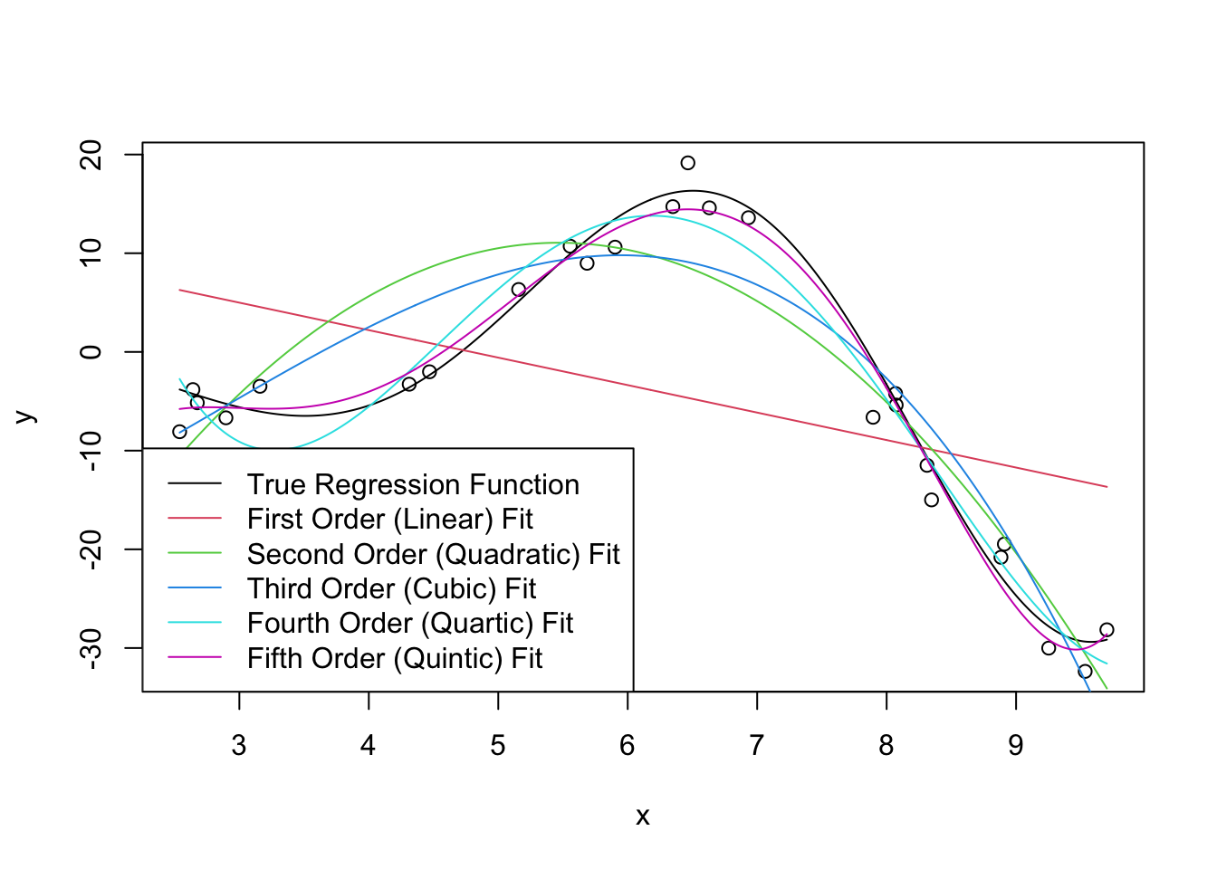

Clearly, as we increase the order of the polynomial, we get a better (in-sample) fit. This makes sense: we know that more features gives us a better fit all else being equal, so what’s the issue?

As usual, the issue occurs for extrapolation. You can actually see some issues already beginning to manifest at the ends of our prediction intervals: the higher-order polynomials go radically different directions as we extrapolate and even the ‘best fit’ (quintic) looks like it’s going to be too steep as we go further.

Let’s expand the prediction region for these fits:

x_pred <- seq(-5, 15, length.out=501)
Ey_pred <- sqrt(abs(x_pred)^3 + 5) * cos(x_pred)
plot(x_pred, Ey_pred, type="l")
points(x, y)

for(k in 1:5){
    m <- lm(y ~ poly(x, k))
    yhat <- predict(m, data.frame(x=x_pred))
    lines(x_pred, yhat, col=k+1)
}

legend("bottomleft",
    c("True Regression Function", 
         "First Order (Linear) Fit",
         "Second Order (Quadratic) Fit", 
         "Third Order (Cubic) Fit", 
         "Fourth Order (Quartic) Fit",
         "Fifth Order (Quintic) Fit"), 
       col=1:6, lty=1)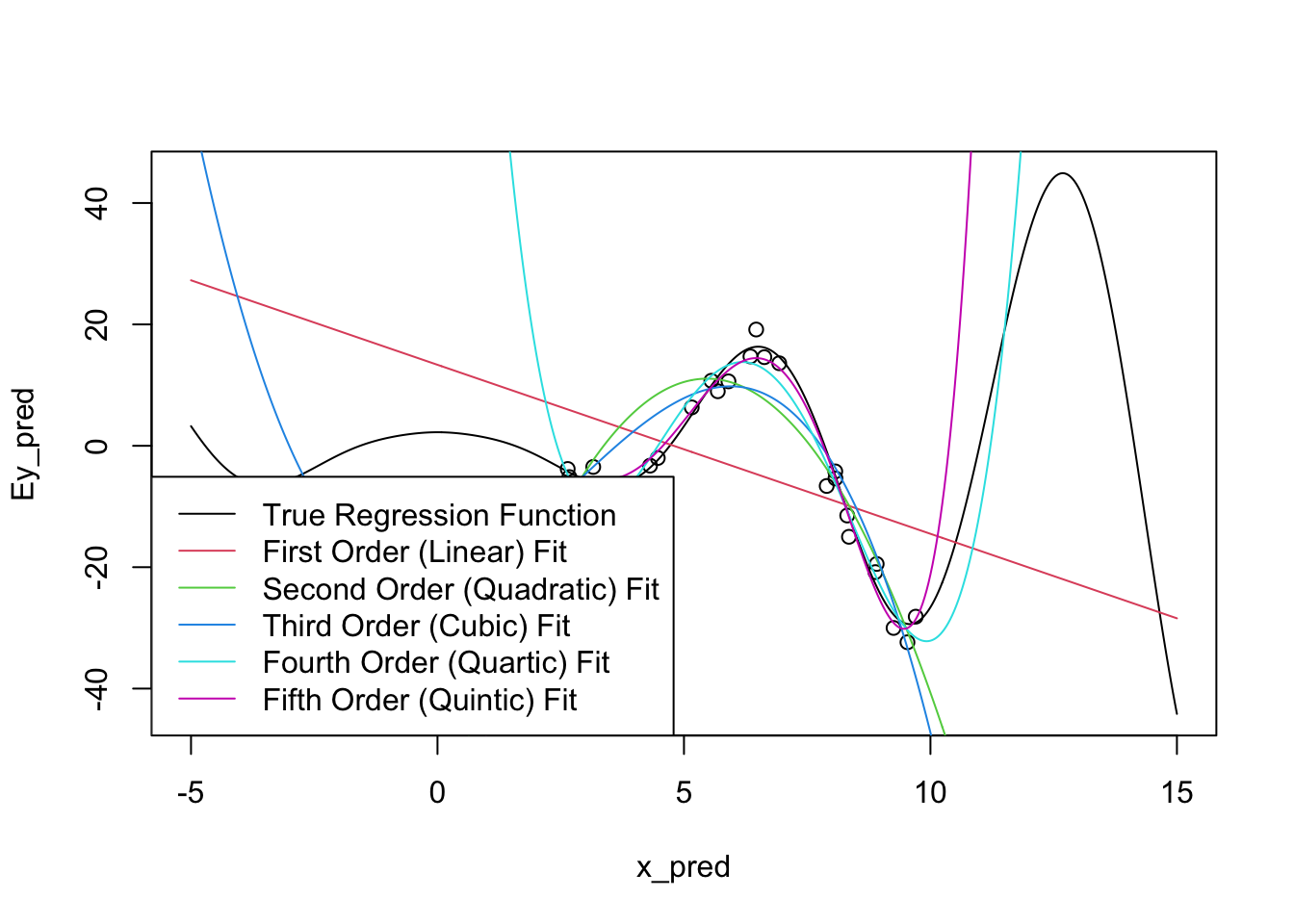

There’s some problems!

To be fair, it is a bit unreasonable to expect these models to perform too well outside of our original sampling area. What’s more worrying is that the extrapolations don’t just miss the curves of the true regression function, they actually create their own even more intense wiggles.

We can also manifest this without extrapolation by fitting very high-order polynomials:

k <- 9
m <- lm(y ~ poly(x, degree=10 + k, raw=TRUE))
yhat <- predict(m, data.frame(x = x_grid))

plot(x, y)
lines(x_grid, Ey_grid)

for(k in 1:5){
    m <- lm(y ~ poly(x, degree=14 + k, raw=TRUE))
    yhat <- predict(m, data.frame(x = x_grid))
    lines(x_grid, yhat, col=k)
}

Note that we have to use raw=TRUE here to avoid R complaining about having too-high a degree in the polynomial. (R gives an error about “unique points” but the real issue is one about matrix rank, not ties in x.) I’m also surpressing some warnings here about a sub-standard fit.

So how can we address this ‘over-wiggliness’?

As we discussed last time, we need to use a different set of functions: one that is smooth (like polynomials), but not too-high order. It would also be really nice if we could get something ‘adaptive’ - allowing for more wiggliness where we have more data (and we need more wiggliness) and less wiggliness where we don’t have enough data (fall-back to linearity). ### Local Linear Models

One way to do this is the idea of “local linear (polynomial) models.” Instead of fitting a single (global) line, we can fit different lines in different parts of our data: that way, we can get an upward line when the true (non-linear) relationship is increasing and a downward line when the true relationship is decreasing. Or at least that’s the hope!

plot(x, y)
lines(x_grid, Ey_grid)

# Divide our data into five 'buckets' and fit sub-models
# This works because we've already sorted our data
# (What would happen if we hadn't?)
for(k in 1:5){
    xk <- x[(5 * k - 4):(5*k)]
    yk <- y[(5 * k - 4):(5*k)]
    mk <- lm(yk ~ xk)
    y_hat <- predict(mk)
    lines(xk, y_hat, col="red4")
}

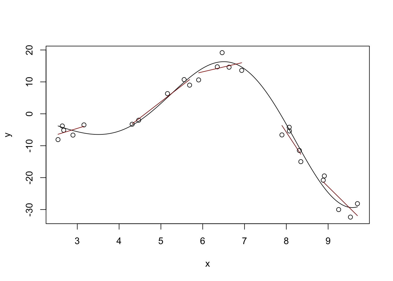
Definitely some rough edges here - particularly in the areas between our buckets, but we’re on a good path. The locfit package will help us with the details:

library(locfit)

locfit 1.5-9.12      2025-03-05


Attaching package: 'locfit'

The following object is masked from 'package:purrr':

    none

m <- (locfit(y ~ lp(x)))
summary(m)

Estimation type: Local Regression 

Call:
locfit(formula = y ~ lp(x))

Number of data points:  25 
Independent variables:  x 
Evaluation structure: Rectangular Tree 
Number of evaluation points:  5 
Degree of fit:  2 
Fitted Degrees of Freedom:  4.848

plot(x, y)
lines(x_grid, Ey_grid)
y_hat <- predict(m, data.frame(x = x_grid))
lines(x_grid, y_hat, col="red4")

Not perfect, but pretty nice compared to what we had before.

You can also see a discussion of the “degrees of freedom” in the model output. This is not exactly the DoF you learned in earlier classes, but it’s sort of “morally equivalent.” This local fit is about as flexible as a 4th degree polynomial would be for this problem. Even though this model is made out of quadratics, it’s more flexible than a single quadratic. But we avoid the extreme variability associated with a polynomial of that high order. Win-win!

We can tweak some parameters of the local fit to get different responses: the big ones are the degree (deg) and the number of neighbors to use.

?lp

m <- (locfit(y ~ lp(x, deg=4)))
summary(m)

Estimation type: Local Regression 

Call:
locfit(formula = y ~ lp(x, deg = 4))

Number of data points:  25 
Independent variables:  x 
Evaluation structure: Rectangular Tree 
Number of evaluation points:  5 
Degree of fit:  4 
Fitted Degrees of Freedom:  6.469

plot(x, y)
lines(x_grid, Ey_grid)
y_hat <- predict(m, data.frame(x = x_grid))
lines(x_grid, y_hat, col="red4")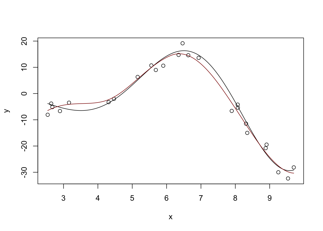

Pretty nice. If we ‘turn down’ the number of neighbors used:

m <- (locfit(y ~ lp(x, nn=0.2, deg=4)))
summary(m)

Estimation type: Local Regression 

Call:
locfit(formula = y ~ lp(x, nn = 0.2, deg = 4))

Number of data points:  25 
Independent variables:  x 
Evaluation structure: Rectangular Tree 
Number of evaluation points:  28 
Degree of fit:  4 
Fitted Degrees of Freedom:  21.586

plot(x, y)
lines(x_grid, Ey_grid)
y_hat <- predict(m, data.frame(x = x_grid))
lines(x_grid, y_hat, col="red4")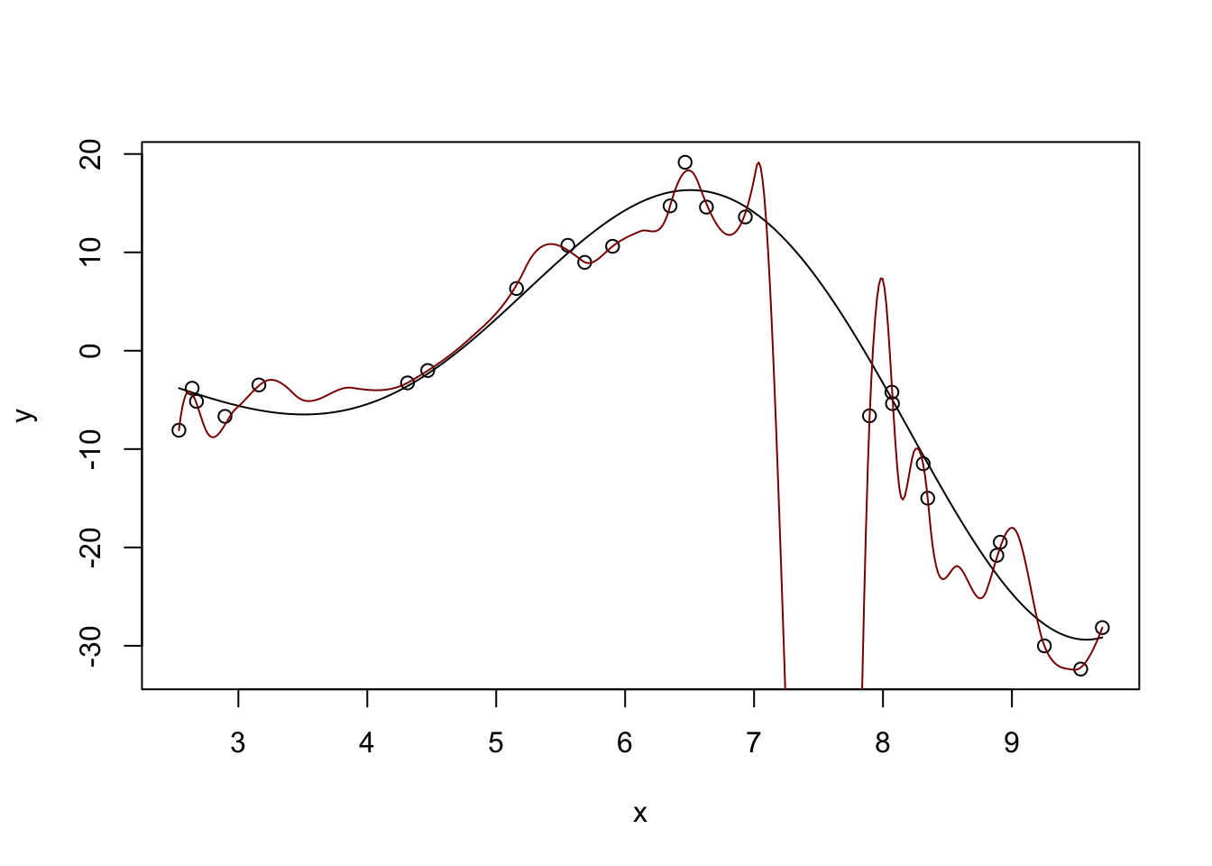

Too far - super crazy! But not entirely unexpected - we know that \(K\)-Nearest Neighbors for small \(K\) has a huge variance.

Too far!

The loess function in base R does this very nicely as well without requiring additional packages. For practical work, it’s a very nice tool for univariate modeling.⁴

m <- loess(y ~ x)
summary(m)

Call:
loess(formula = y ~ x)

Number of Observations: 25 
Equivalent Number of Parameters: 4.41 
Residual Standard Error: 2.846 
Trace of smoother matrix: 4.84  (exact)

Control settings:
  span     :  0.75 
  degree   :  2 
  family   :  gaussian
  surface  :  interpolate     cell = 0.2
  normalize:  TRUE
 parametric:  FALSE
drop.square:  FALSE

plot(x, y)
lines(x_grid, Ey_grid)
y_hat <- predict(m, data.frame(x = x_grid))
lines(x_grid, y_hat, col="red4")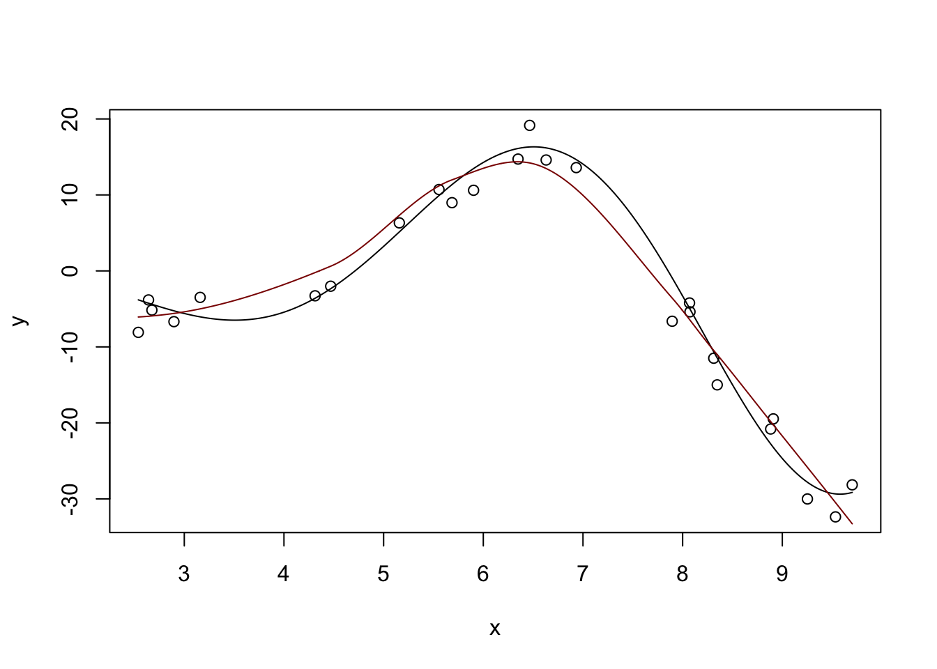

Spline Regression (Additive Models)

Splines

We can generalize this idea a bit using splines. Splines are functions that solve a penalized approximation problem:

\[\hat{f} = \argmin_{f} \frac{1}{2n} \|y - f(x)\|_2^2 + \lambda \int |f''(x)|^2 \text{d}x\]

Here we are saying we’ll take any function (not just a polynomial) that achieves the optimal trade-off between data fit (first / loss term) and not being too rough (second / penalty term).

Why is this the right penalty to use? In essence, we are trying to penalize ‘deviation from linearity’ and since linear functions have second derivative 0 (by definition) the integral of the second derivative gives us a measure of non-linearity.

In some remarkable work, Grace Wahba and co-authors showed that the solutions to that optimization problem are piecewise polynomials with a few additional constraints - these functions are splines. In addition to piecewise polynomialness, splines also guarantee:

continuity of the function and its derivatives
linearity outside the range of data fit (‘natural splines’)

Because splines not only match the value of the function at the knots (places where the ‘pieces’ match up) but also the derivatives, they are very smooth indeed.

Stepping back, splines are just a different sort of feature engineering. Instead of using polynomial basis functions (\(x^1, x^2, \dots, x^k\)), splines use a much smoother basis and hence give smoother results, avoiding the ‘wiggles’ problem we saw above.

R provides the basic tools for spline fitting in the splines package. For real work, you almost surely want to use the advanced functionality of the mgcv package. For more on splines and models using them (‘additive models’), see this online course.

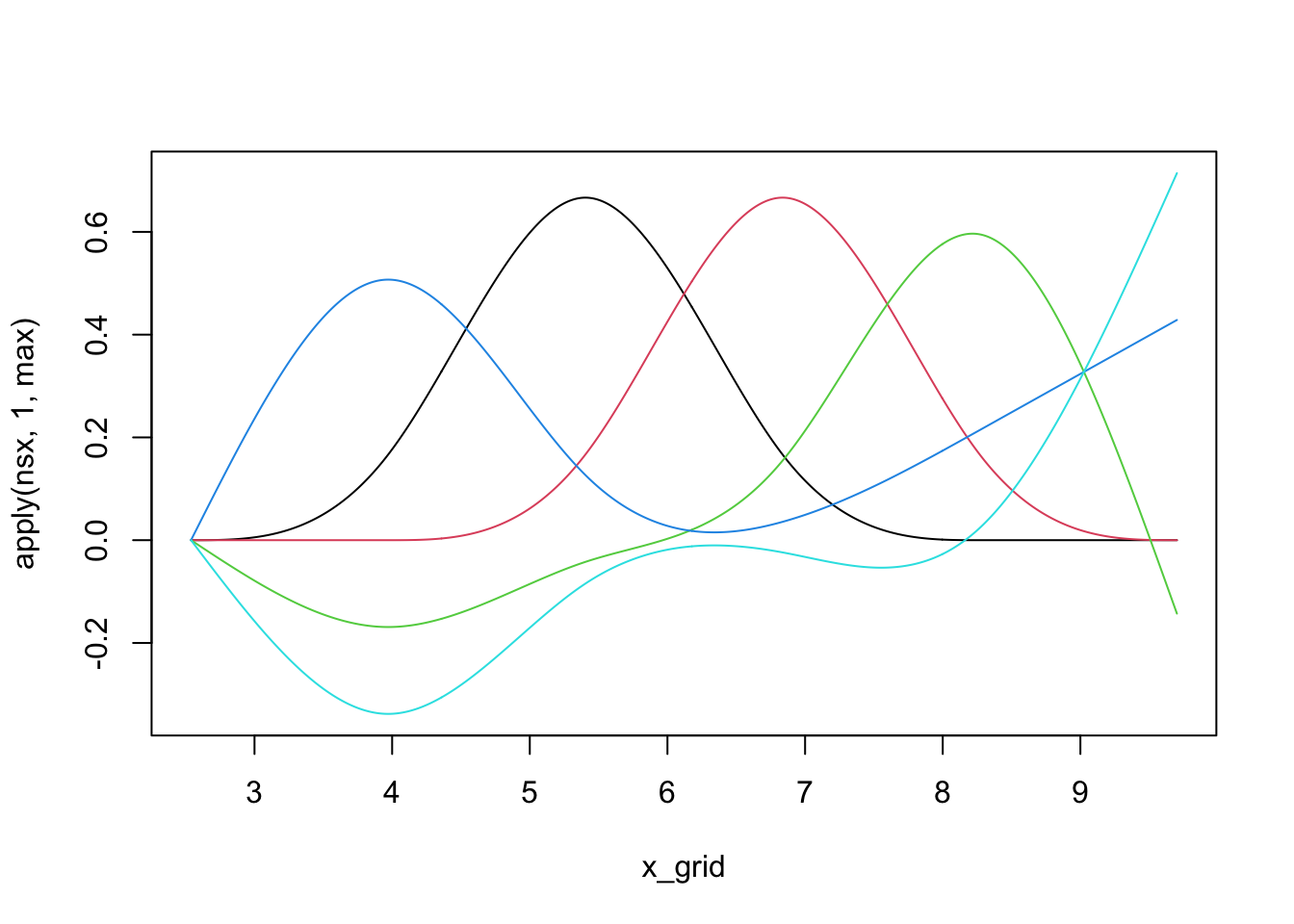
We can see that individual splines are quite nice little functions and usually are only non-zero on small regions:

library(splines)

nsx <- ns(x_grid, df=5) # The natural spline basis
plot(x_grid, apply(nsx, 1, max), ylim=range(nsx), type="n")

for(i in 1:5){
    lines(x_grid, nsx[,i], col=i)
}

We can use linear combinations of these ‘bumps’ to fit non-linear functions, including our example from above:

m <- lm(y ~ ns(x, df=5))
plot(x, y)
lines(x_grid, Ey_grid)
y_hat <- predict(m, data.frame(x = x_grid))
lines(x_grid, y_hat, col="red4")

(This basically matches what we had before with \(\text{DoF} \approx 4.7\), but you can get different answers by messing with the df parameter here.)

Our predicted response is actually the sum of the individual spline effects:

m <- lm(y ~ ns(x, df=5))
y_hat <- predict(m, data.frame(x = x_grid))

plot(x, y, lwd=2)
lines(x_grid, Ey_grid)
for(i in 1:5){
    lines(x_grid, ns(x_grid, df=5)[,i] * coef(m)[-1][i], col=i+1)
}

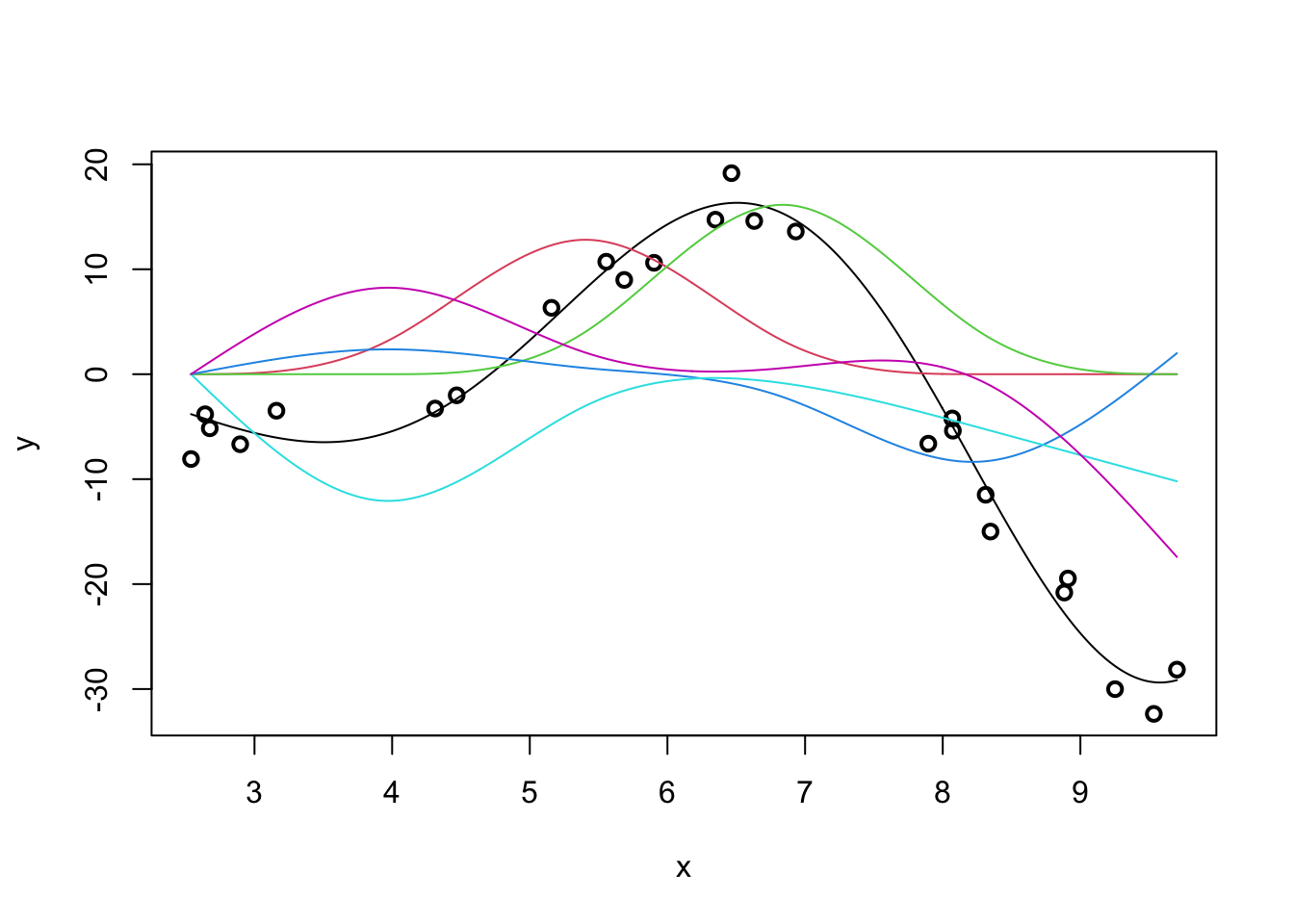
If we were able to sum up the colored lines, we would get the black line back.

We can also see that natural splines give smooth predictions outside the range of the original data:

y_pred <- predict(m, data.frame(x = x_pred))

plot(x_pred, Ey_pred, type="l")
lines(x_pred, y_pred, col="red4")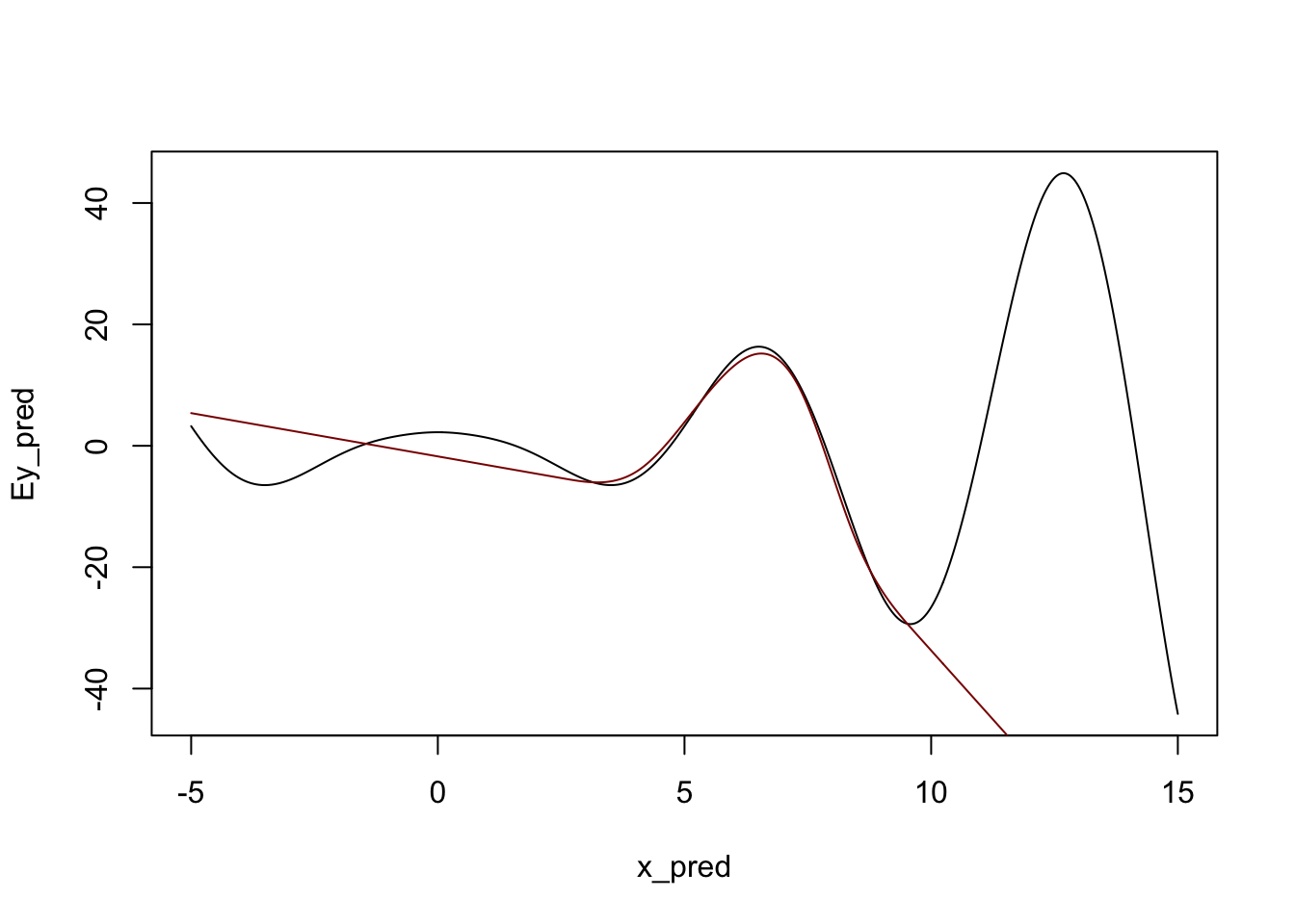

Admittedly, not ideal, but it will do. In particular, note that outside of the ‘data region’, we fall back on a nice comfortable

(You can repeat this process with the slightly more common \(b\)-splines, but the differences aren’t huge.)

m <- lm(y ~ bs(x, df=5))
y_hat <- predict(m, data.frame(x = x_grid))

plot(x, y, xlim=range(x_grid))
lines(x_grid, Ey_grid)
for(i in 1:5){
    lines(x_grid, bs(x_grid, df=5)[,i] * coef(m)[-1][i], col=i+1)
}

y_pred <- predict(m, data.frame(x = x_grid))

lines(x_grid, y_pred, col="red4", lwd=2)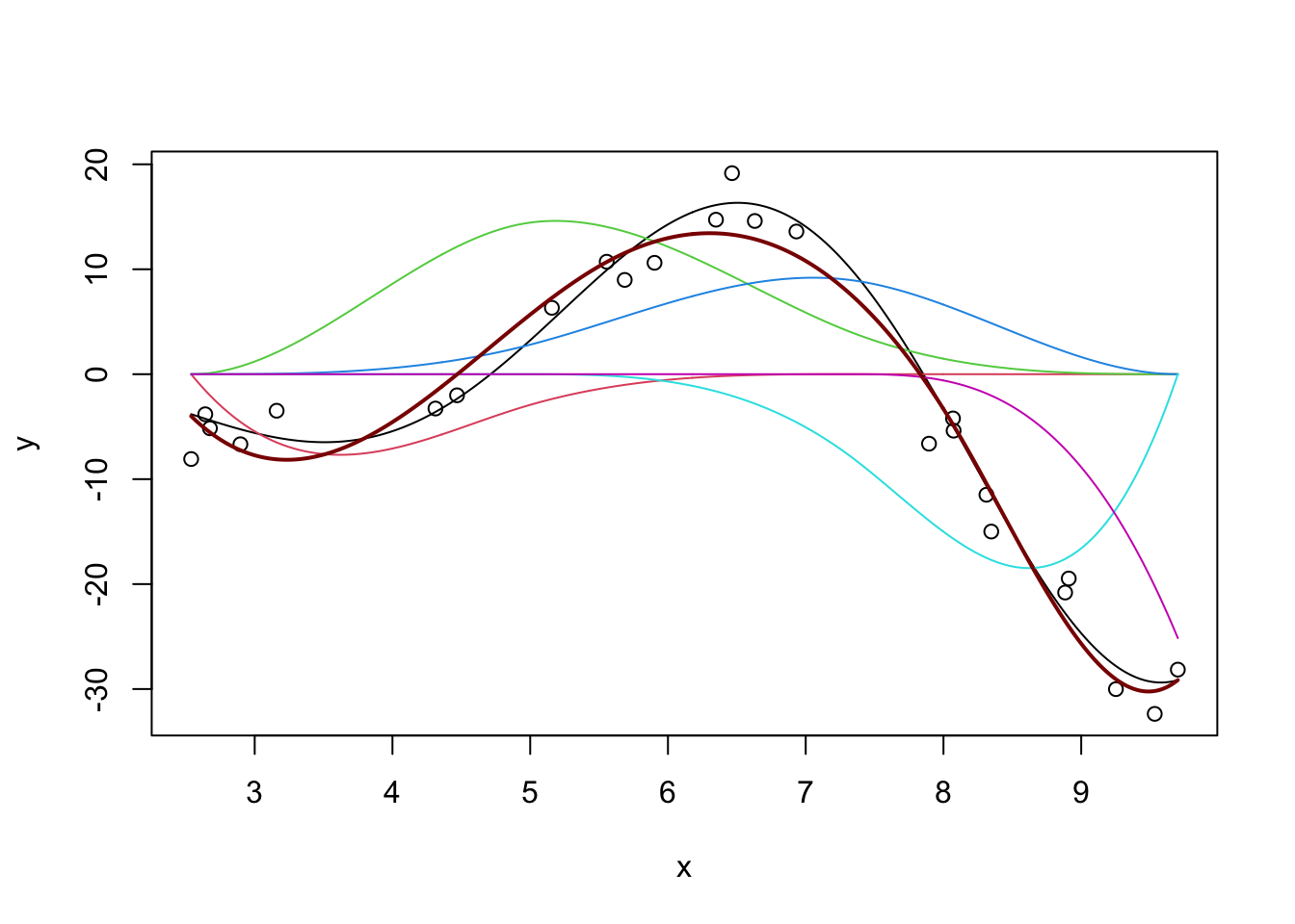

For a ‘full-strength’ version of spline fitting, you can use the mgcv package:

library(mgcv)

Loading required package: nlme


Attaching package: 'nlme'

The following object is masked from 'package:dplyr':

    collapse

This is mgcv 1.9-3. For overview type 'help("mgcv-package")'.


Attaching package: 'mgcv'

The following object is masked from 'package:locfit':

    lp

m <- gam(y ~ s(x))

summary(m)


Family: gaussian 
Link function: identity 

Formula:
y ~ s(x)

Parametric coefficients:
            Estimate Std. Error t value Pr(>|t|)    
(Intercept)  -4.2915     0.4823  -8.898 4.78e-08 ***
---
Signif. codes:  0 '***' 0.001 '**' 0.01 '*' 0.05 '.' 0.1 ' ' 1

Approximate significance of smooth terms:
       edf Ref.df     F p-value    
s(x) 5.808  6.925 121.4  <2e-16 ***
---
Signif. codes:  0 '***' 0.001 '**' 0.01 '*' 0.05 '.' 0.1 ' ' 1

R-sq.(adj) =  0.972   Deviance explained = 97.9%
GCV = 7.9909  Scale est. = 5.8149    n = 25

m <- gam(y ~ s(x))
y_hat <- predict(m, data.frame(x = x_grid))

plot(x, y, xlim=range(x_grid))
lines(x_grid, Ey_grid)
lines(x_grid, y_hat, col="red4", lwd=2)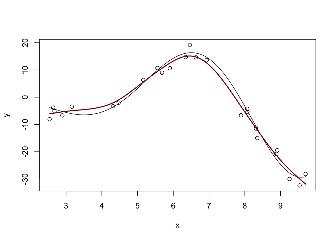

Run ?s to see the many features of the mgcv package. mgcv also includes several specialized splines (e.g. periodic) which you may find useful in some problems.

Splines are not normally consider a ‘machine learning’ tool but they are incredibly useful in applied statistics work. (The two methods you will rely on most from this class are spline regression and random forests.)

\(\ell_1\)-Filtering

Kernel Methods

Manual feature expansion

We can think of feature expansion as mapping our data to a higher-dimensional space \(\Phi: \R^p \to \R^P\) and fitting a linear model there. As we have seen above, splines and their kin provide a useful way of constructing the mapping \(\Phi\), but we are still constrained to work with a fairly restricted type of problem.

Can we generalize this formally to more interesting maps \(\Phi(\cdot)\)? Yes - via kernel methods!

Ridge without coefficients

Before introducing kernel methods formally, let’s look back to ridge regression. We showed that the ridge solution is given by

\[\hat{\beta}_{\text{Ridge}} = (\bX^T\bX + \lambda \bI)^{-1}(\bX^T\by)\]

Some nifty linear algebra will let us rewrite this as

\[\hat{\beta}_{\text{Ridge}} = \lambda^{-1}\bX^T(\bX\bX^{\top}/\lambda + \bI)^{-1}\by = \bX^{\top}(\bX\bX^{\top}+\lambda \bI)^{-1}\by\]

You can prove this using the Woodbury Matrix Identity or we can just check it for a single data set and trust that it generalizes:

n <- 100
p <- 5 

X <- matrix(rnorm(n * p), nrow=n, ncol=p) 

Ey <- X[,1] + sqrt(X[,2]^2 + 5) + 0.1 * X[,3]^3 + cos(abs(X[,4])) + 1/(abs(X[,5]) + 3)
y <- Ey + rnorm(n, sd=sqrt(0.25))

lambda <- 2
eye <- function(p) diag(1, p, p)
beta_hat_ridge <- solve(crossprod(X) + lambda * eye(p), crossprod(X, y))

beta_hat_ridge_alt <- t(X) %*% solve(tcrossprod(X) + lambda * eye(n)) %*% y

cbind(beta_hat_ridge, beta_hat_ridge_alt)

           [,1]       [,2]
[1,]  1.1679876  1.1679876
[2,]  0.2056050  0.2056050
[3,]  0.7831282  0.7831282
[4,]  0.5725460  0.5725460
[5,] -0.1197009 -0.1197009

So they are the same! But why did we do this?

It is sometimes a bit more computationally efficient if we have to invert an \(n \times n\) matrix instead of a \(p \times p\) matrix, but there are faster methods if we’re really interested in speed.

Note that, if we want to make a ridge regression prediction now for a new \(\tilde{\bx}\), we just need to compute:

\[\begin{align*} \hat{\beta}_{\text{Ridge}}^T\tilde{\bx} &= \left[\bX^{\top}(\bX\bX^{\top}+\lambda \bI)^{-1}\by\right]^T\tilde{\bx} \\ &= \left[\by^T(\bX\bX^{\top}+\lambda \bI)^{-T}\bX\right]\tilde{\bx} \\ &= \by^T(\bX\bX^{\top}+\lambda \bI)^{-1} \bX\tilde{\bx} \end{align*}\]

Intuitively, recall that the inner product of two vectors measures the angle between them and can, up to some scaling, be used as a ‘similarity’ measure. This result essentially says that our prediction on a new data set is a weighted average of the training data, with weights based on similarity of the new point with the training data. This is not a crazy structure…

If we look closer, we see that we only need to compute products of the form \(\bx_1\bx_2\) to make this work. This is where the magic of kernels lies.

Kernel Trick

Earlier, we considered non-linear regression by feature expansion, where we replaced \(\bX\) by \(\Phi(\bX)\), where \(\Phi: \R^p \to \R^P\) maps to a higher-dimensional space (applied row-wise). We can use this mapping in our new ridge formula to get our non-linear predictions as

\[\begin{align*} \hat{y}(\tilde{\bx}) &= \by^T(\Phi(\bX)\Phi(\bX)^{\top}+\lambda \bI)^{-1} \Phi(\bX)\Phi(\tilde{\bx}) \end{align*}\]

Longer, but not necessarily better. If \(P\) is very large, computing with \(\Phi(X)\) can be incredibly expensive.

It turns out, however, that we never need to actually form \(\Phi(X)\), we only need \(\kappa(\bx_1, \bx_2) = \Phi(\bx_1)^T\Phi(\bx_2)\). If we can compute \(\kappa\) directly, we never need to work with \(\Phi\).

Functions that allow this are called (Mercer) kernels and they are just a little bit magical.

If we let \(\K = \Phi(X)\Phi(X)^{\top}\) be defined by \(\K_{ij} = \kappa(\bx_i, \bx_j)\), then we can write our feature-augmented ridge regression as:

\[\hat{y}(\tilde{\bx}) = \by^T(\K+\lambda \bI)^{-1} \kappa(\bX, \tilde{\bx})\]

If we break this apart, we see that our predictions at the new point \(\tilde{\bx}\) are essentially just weighted averages of our original observations \(\by\), weighted by the similarity between the new point and our training points \(\kappa(\bX, \cdot)\). This intuition is super important and we’ll dig into it further below.

Let’s try out Kernel(ized) Ridge Regression:

library(kernlab)


Attaching package: 'kernlab'

The following object is masked from 'package:CVXR':

    size

The following object is masked from 'package:purrr':

    cross

The following object is masked from 'package:ggplot2':

    alpha

## Define a kernel function - we'll spell this out below.
rbf <- rbfdot(sigma = 0.05)

## calculate kernel matrix
K <- kernelMatrix(rbf, X)
dim(K)

[1] 100 100

Note that this is a \(n \times n\) matrix - not a \(p \times p\) matrix!

We can now use this to make predictions:

krr <- function(x, lambda=1) {
    crossprod(y, solve(K + lambda * eye(n), kernelMatrix(rbf, X, x)))
}

krr_MSE <- mean((y - krr(X))^2)
print(krr_MSE)

[1] 0.4680494

This is better than the OLS MSE:

mean(resid(lm(y ~ X))^2)

[1] 0.4151421

Why? How is this not a contradiction of everything said before.

But how do we actually do kernel multiplication?

There are many kernel functions in the world. The most common are defined by:

\(\kappa(\bx_1, \bx_2) = \bx_1^{\top}\bx_2\). This is the linear kernel, equivalent to non-kernel methods
\(\kappa(\bx_1, \bx_2) = (\bx_1^{\top}\bx_2 + c)^d\). This is the polynomial kernel, equivalent to fitting polynomial regression up to degree \(d\) with all cross products. (The role of \(c\) is tricky, but it essentially controls the relative weight of the higher and lower order terms)
\(\kappa(\bx_1, \bx_2) = e^{-\sigma^2\|\bx_1 - \bx_2\|^2}\). This is the squared exponential or radial basis function (RBF) kernel; it is very popular in spatial statistics, where it is closely related to a method known as kriging.

While the first two kernels give us a natural \(\Phi(\cdot)\) mapping, the \(\Phi(\cdot)\) for the RBF kernel is actually infinite dimensional: it lets us fit function classes we could not fit without the kernel trick.

For even more kernels, see:

Much of our current understanding of deep learning is based on specialized kernel methods:

The Neural Tangent Kernel
Kernel Methods for Deep Learning
Gradient Descent as a Kernel Machine (This paper is a bit controversial)

This blog is a particularly nice (but still somewhat technical) introduction to the Neural Tangent Kernel and its relationship to neural networks.

Spline theory has also found use to explain ReLU (piecewise linear activation) neural networks:

We can also kernelize some of the other methods we’ve studied in this course.

Notably, we can kernelize \(K\)-Nearest Neighbors to get “KKNN” if we modify the definition of distance used to be “kernel-ish.” We first recall that we can write distances solely in terms of inner products:

\[\begin{align*} \|\bx_1 - \bx_2\|_2^2 &= (\bx_1 - \bx_2)^T(\bx_1 - \bx_2) \\ &= \bx_1^T\bx_1 - \bx_2^T\bx_1 - \bx_1^T\bx_2 + \bx_2^T\bx_2 \\ &= \bx_1^T\bx_1 - 2\bx_1^T\bx_2 + \bx_2^T\bx_2 \\ \implies \text{Kernel Distances} &= \kappa(\bx_1, \bx_1) - 2\kappa(\bx_1, \bx_2) + \kappa(\bx_2, \bx_2) \end{align*}\]

If we compute distances this way for a given \(\kappa\), we get kernel KNN. This is particularly nice when we have kernels that capture specific behaviors (e.g., periodic or embedded categorical) that we can’t really treat as Euclidean.

Trade-Offs between Linear and Non-Linear Methods

Having developed some tools for non-linear regression, let’s step back and ask whether they are worthwhile. Recall our error decomposition:

\[\MSE = \text{Irreducible Error} + \text{Variance} + \text{Model Bias}^2 + \text{Estimation Bias}^2\]

We have already discussed how tools like ridge and lasso let us remove variance at the cost of (estimation) bias.

We argued that this was a worthwhile trade when the problem had a lot of ‘innate’ variance, either from having large noise variance (\(\V[\epsilon] \gg 0\)) or from having many features. In particular, use of some sort of shrinkage (ridge or lasso penalization) was essential in the ‘high-dimensional’ case (\(p > n\)) where OLS had so much variance that it was not even uniquely defined. We also argued that, as we got more and more data (\(n \to \infty\)), the variance took care of itself in the usual statistical way.

These lessons generalize to the non-linear vs linear debate as well. Choosing to use a linear model is itself a variance reducing choice - there are ‘more’ curves than lines in some sense. If we restrict our attention to linear models only, we are potentially accepting some Model Bias, again with a hope of reducing variance to get overall better performance. As such, the same intuition as above applies: linear models are preferred when variance is the primary concern, either from noisy data or from small data; as we get more data, variance decreases naturally, so going to non-linear models reduces bias, giving overall smaller error.

In the non-linear context, the ‘estimation bias / variance’ trade-off remains, but modern tools like mgcv essentially handle this automatically for us. It is of course still there, but mgcv has some nifty auto-tuning built-in.⁵

Footnotes

For historical reasons, this is known as the inverse link, but I prefer to simply think of it as an adaptor and to never use the (forward) link.↩︎
This ‘surrogate loss’ perspective was first discussed in: P.L. Barlett, M.I. Jordan, and J.D. McAuliffe. “Convexity, Classification, and Risk Bounds”. Journal of the American Statistical Association 101(473), pp.138-156. 2006. DOI:10.1198/016214505000000907 ↩︎
In other classes, you may have been taught that polynomial regression is a linear model. It is definitely linear in the sense that that class would have used (linear in \(\by\)) but we’re using a different sense here. The core insight of that analysis - that a non-linear function can be expressed as a linear combination of non-linear parts - will appear several times in these notes.↩︎
In Python, the statsmodels package also implements LOESS fits.↩︎
If you want to go much deeper into the practical use of additive (spline) models, Simon Wood’s book Generalized Additive Models is fantastic.↩︎

STA 9890 - Supervised Learning: IV. Discriminative Classifiers & Non-Linear Methods

Discriminative Classifiers

Why Not Accuracy Maximization?

OLS for Classification?

Deriving Logistic Regression

From Model to Loss Function

Generalized Linear Models

Loss Functions for Classification

Support Vector Machines

SVM: The Geometric Viewpoint

Non-Linear Methods

Non-Linearity via Linear Combination of Non-Linear Parts

Polynomial Expansion

Spline Regression (Additive Models)

Splines

\(\ell_1\)-Filtering

Kernel Methods

Manual feature expansion

Ridge without coefficients

Kernel Trick

Trade-Offs between Linear and Non-Linear Methods

Other Topics in Regression

Alternative Loss Functions

Multi-Task Regression

Weights and generalization

Footnotes