STA 9890 - Unsupervised Learning: III. Linear Dimension Reduction

Author

Michael Weylandt

Published

May 6, 2026

\[\newcommand{\R}{\mathbb{R}} \newcommand{\E}{\mathbb{E}} \newcommand{\V}{\mathbb{V}} \newcommand{\P}{\mathbb{P}} \newcommand{\C}{\mathbb{C}} \newcommand{\bbeta}{\mathbb{\beta}} \newcommand{\bone}{\mathbf{1}} \newcommand{\bzero}{\mathbf{0}} \newcommand{\ba}{\mathbf{a}} \newcommand{\bb}{\mathbf{b}} \newcommand{\bc}{\mathbf{c}} \newcommand{\bv}{\mathbf{v}} \newcommand{\br}{\mathbf{r}} \newcommand{\bw}{\mathbf{w}} \newcommand{\bx}{\mathbf{x}} \newcommand{\by}{\mathbf{y}} \newcommand{\bz}{\mathbf{z}} \newcommand{\bX}{\mathbf{X}} \newcommand{\bA}{\mathbf{A}} \newcommand{\bB}{\mathbf{B}} \newcommand{\bC}{\mathbf{C}} \newcommand{\bD}{\mathbf{D}} \newcommand{\bu}{\mathbf{u}} \newcommand{\bU}{\mathbf{U}} \newcommand{\bV}{\mathbf{V}} \newcommand{\bI}{\mathbf{I}} \newcommand{\bH}{\mathbf{H}} \newcommand{\bW}{\mathbf{W}} \newcommand{\bK}{\mathbf{K}} \newcommand{\bR}{\mathbf{R}} \newcommand{\argmin}{\text{arg\,min}} \newcommand{\argmax}{\text{arg\,max}} \newcommand{\MSE}{\text{MSE}} \newcommand{\Fcal}{\mathcal{F}} \newcommand{\Dcal}{\mathcal{D}} \newcommand{\Ycal}{\mathcal{Y}} \newcommand{\Ocal}{\mathcal{O}} \newcommand{\bv}{\mathbf{v}} \newcommand{\Tr}{\text{Tr}}\]

Today, we begin our study of dimension reduction, the task of finding a simplified representation of your data. Before we begin formalizing DR, it is worthwhile to take a second to think about why we may want to perform DR as this will help us design suitable loss functions.

For now, let’s take DR ‘literally’ and assume that we’re trying to find a lower-dimensional representation: that is, given data points \(\bx_i \in \R^P\), we want to find \(\bx_i \in \R^p\) for some \(p \ll P\).¹ Typically, \(P\) may be \(\Ocal(1000-10000)\) and \(p\) will be \(\Ocal(1-10)\). To identify the goals of DR, let’s think about the problems associated with large \(P\):

Difficult data exploration and visualization
- Our standard tools, like a scatter plot or a ‘pairs plot’, simply aren’t feasible for large dimensions. Even if we lean into tools like ggplot, we really can only plot 5-6 dimensions at a time (\(x\), \(y\), size, color, shape, 2 facets)
Interpretation
- We can’t really make sense of data with several thousand features. There will be significant correlation among features (even if just ‘by chance’) and finding ‘important’ features as opposed to ‘noise’ features becomes essentially impossible (even ignoring the definition issues)
Supervised Learning
- Building supervised models with \(P\) features is harder than building models with \(p\) features, particuarly if we are prioritizing interpretability. While we have developed techniques that prioritize interpretation in some methods (lasso and variants for linear regression), these are somewhat special purpose and can’t be applied to arbitrary learning methods.

Clearly, in each of these, we’re going to have an easier time if we only have \(p\) features. And we could get \(p\) features quite easily by simply ‘throwing away’ most of our variables… But this has a rather obvious problem: if we throw away features willy-nilly, we might throw away the important ‘signal’ components of our data. So we want to build a model for automatically mapping from \(\R^P\) to \(\R^p\) that keeps the ‘signal’ (as best as we can estimate it).

Of course, this requires us to make the concept of ‘signal’ mathematically precise. We might consider goals like the following:

‘Distance preservation’: if \(\bx, \by \in \R^P\) are far apart, we want \(f(\bx), f(\by) \in \R^p\) to be far aapart as well. Similarly, if two points \(\bx, \by \in \R^P\) are close, we want their DR’d points \(f(\bx), f(\by)\) to be close in the reduced space.
‘Angle preservation’: if \(\bx, \by \in \R^p\) are at an angle of approximately \(\theta\), we want the angle between \(f(\bx)\) and \(f(\by)\) to be similar. In particular, if \(\bx, \by\) are orthogonal, we want \(f(\bx), f(\by)\) to be orthogonal as well.

Mathematically, it will suffice to maintain inner products, as inner products generate distances and angles: that is, we want

\[\langle \bx, \by \rangle_{\R^P} \approx \langle f(\bx), f(\by) \rangle_{\R^p}\]

If you prefer a more statistical (as opposed to geometric) motivation, you can think of our desiderata as maintaining variances (distances) and correlations (angles) among aspects of our data: clearly, it suffices to maintain covariances (inner products).

PCA: First Steps

So, with that goal in mind, let’s start building our first dimension reduction technique. Consistent with our treatment of unsupervised learning, we’ll begin by assuming \(f\) is a linear operation and living in the world of MSE. As we build our method, let’s start by taking \(p=1\) (reducing down to a single dimension) but we’ll relax this in a bit.

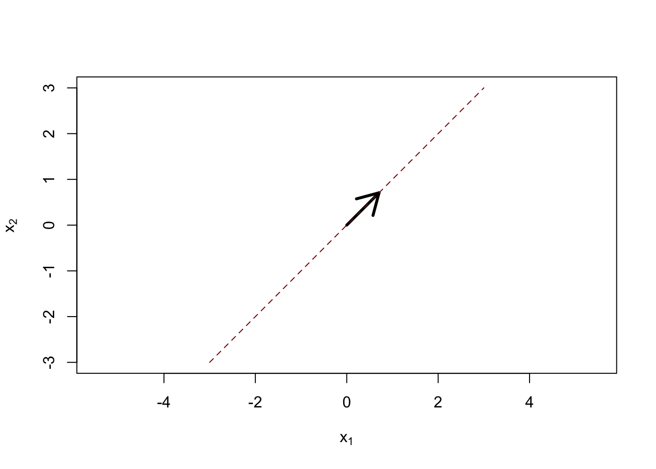
Our reduced dimension space can be parameterized by a single vector \(\bv \in \R^P\), with the reduced space being defined by \[\textsf{Span}(\bv) = \{\lambda \bv: \lambda \in \R\}.\] That is, our reduced space is the line generated by \(\bv\):

Here the black arrow is \(\bv\) and the dashed red line is \(\textsf{Span}(\bv)\). For a given space, the choice of \(\bv\) is clearly not unique: if we streteched or even flipped \(\bv\), \(\textsf{Span}(\bv)\) would remain unchanged, so we might as well assume \(\|\bv\|=1\) without loss of generality.

Once we have \(\bv\), how can we actually build the mapping \(f(\cdot): \R^P \to \textsf{Span}(\bv)\)? Well, if our goal is to minimize MSE, it makes sense to find the point in \(\textsf{Span}(\bv)\) that lies closest to our original point. It’s hopefully not too hard to convince yourself that this point is given by the projection of \(\bx\) onto \(\textsf{Span}(\bv)\), which is given by

\[\bv \frac{\langle \bx, \bv \rangle}{\langle \bv, \bv\rangle} = \langle \bx, \bv\rangle \bv = \bx^{\top}\bv \bv\]

Visually:

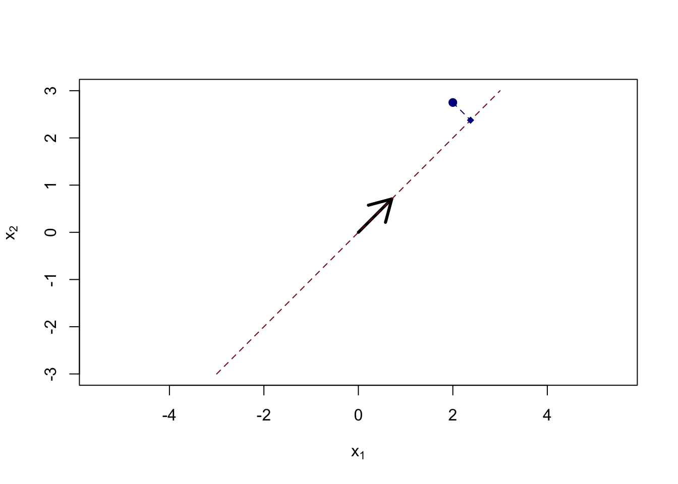
Here, we have projected the original point (big blue) to the nearest point on \(\textsf{Span}(\bv)\) (red dashed line), resulting in the DR’d smaller blue point. The ‘loss’ of this projection is measured by the Euclidean distance between the two points, here captured by the dashed blue line.

We note here that the relevant distance here is the perpendicular (straight line) distance from the original point to the target space. We do not make the \(y\)-axis special, unlike supervised learning where there is a ‘special’ response variable.

With this in hand, we are now ready to define the loss function we use to select \(v\):

\[\argmin_{\bv: \|\bv\|==1} \left\|\bx - \textsf{proj}_{\textsf{Span}(\bv)}(\bx)\right\|_2^2 = \argmin_{\bv: \|\bv\|==1} \left\|\bx - \bv \langle \bx, bv\rangle\right\|_2^2 = \argmin_{\bv: \|\bv\|==1} \left\|\bx - \bx^{\top}\bv \bv\right\|_2^2 \]

With many training points, our problem generalizes to the sum of total errors, giving us:

\[ \argmin_{\bv: \|\bv\|==1} \sum_i \left\|\bx_i - \bx^{\top}_i\bv \bv\right\|_2^2 = \argmin_{\bv: \|\bv\|==1} \left\|\bX - \bX\bv\bv^{\top}\right\|_F^2 = \argmin_{\bv: \|\bv\|==1} \left\|\bX(\bI - \bv\bv^{\top})\right\|_F^2\]

Looking at this, we see a certain similarity to OLS: we are using \(\bX\) to predict the projected \(\bX\) in a minimum MSE sense. But, unlike standard supervised learning where the response is fixed, here we get to select the response (indirectly by selecting \(\bv\)) that makes the problem as easy as possible (i.e., we get to pick the response so that the final residuals are as small as possible).

In this sense DR is a self-supervised problem: we are finding a projection that is the most predictable and looses the least amount of variance in \(\bX\). This actually ties unsupervised learning to supervised learning nicely: in supervised learning, we want to find reliable accurate predictions. In unsupervised learning, we don’t have a sense of prediction and are instead settling for finding a ‘repeatable’ pattern. But, if the pattern we find corresponds to a reliable and accurate prediction, it’s not unreasonable to assume it will generalize out-of-sample in some sense.

So how can we actually solve this problem? It’s not as clean as OLS since \(\bv\) gets ‘squared’ inside the loss (giving a fourth-degree polynomial in \(\bv\)), but it will turn out to be quite solvable anyways. If we expand our our loss, we get the following:

\[\begin{align*} \left\|\bX - \bX\bv\bv^{\top}\right\|_F^2 &= \left\|\bX\right\|_F^2 - 2 \langle \bX, \bX\bv\bv^{\top}\rangle + \left\|\bX\bv\bv^{\top}\right\|_F^2\\ &= \left\|\bX\right\|_F^2 - 2 \langle \bX, \bX\bv\bv^{\top}\rangle + \langle\bX\bv\bv^{\top}, \bX\bv\bv^{\top}\rangle\\ &= \left\|\bX\right\|_F^2 - 2 \Tr(\bX^{\top}\bX\bv\bv^{\top})+ \Tr((\bX\bv\bv^{\top})^{\top}(\bX\bv\bv^{\top})) \\ &= \left\|\bX\right\|_F^2 - 2 \Tr(\bv^{\top}\bX^{\top}\bX\bv)+ \Tr(\bv\bv^{\top}\bX^{\top}\bX\bv\bv^{\top}) \\ &= \left\|\bX\right\|_F^2 - 2 \Tr(\bv^{\top}\bX^{\top}\bX\bv)+ \Tr(\bv^{\top}\bX^{\top}\bX\bv\underbrace{\bv^{\top}\bv}_{=\|\bv\|^2=1}) \\ &= \left\|\bX\right\|_F^2 - 2 \Tr(\bv^{\top}\bX^{\top}\bX\bv)+ \Tr(\bv^{\top}\bX^{\top}\bX\bv) \\ &= \left\|\bX\right\|_F^2 - \Tr(\bv^{\top}\bX^{\top}\bX\bv) \\ &= \left\|\bX\right\|_F^2 - \bv^{\top}\bX^{\top}\bX\bv \end{align*}\] Because \(\|\bX\|_F^2\) doesn’t change as a function of \(\bv\), this means our problem can be reduced to

\[\argmin_{\bv: \|\bv\|=1} - \bv^{\top}\bX^{\top}\bX\bv = \argmax_{\bv: \|\bv\|=1} \bv^{\top}\bX^{\top}\bX\bv\]

We see here that the \(\|\bv\|=1\) constraint is important: if this constraint was missing, we could simply make the objective arbitrarily large by increasing \(\bv\) without limit.

This gives us our second interpretation of our DR problem:

We want to minimize the loss in projecting \(\bX\) into \(\textsf{Span}(\bv)\)
We want to maximize the amount of \(\bX^{\top}\bX\) captured in the \(\bv\) direction.

At this point, it is perhaps with noting that the DR problem we have developed (in whatever form you prefer) is Principal Components Analysis (PCA).

Solving the PCA Problem with Linear Matrix Decompositions

So how can we solve the PCA problem?

\[\argmax_{\bv: \|\bv\|=1} \bv^{\top}\bX^{\top}\bX\bv\]

While you might be tempted to use the tools of convex optimization here, this isn’t actually a convex problem. In particular, we’re looking to maximize, while convex optimization normally lets us minimize. So we need to return to first principles:

We might first consider using a gradient ascent method, modifying it to maintain our \(\|\bv\|=1\) constraint. In particular, if we differentiate \(\bv^{\top}\bX^{\top}\bX\bv\) with respect to \(\bv\), we get \(2\bX^{\top}\bX\bv\), so an iteration like

\[ \bv^{(k+1)} \leftarrow \bv^{(k)} + c 2\bX^{\top}\bX\bv^{(k)} = (\bI + 2c\bX^{\top}\bX)\bv^{(k)}\]

might make sense. Rather than selecting the step size \(c\) directly, we can instead assume that we want to as far as we can without violating the \(\|\bv\|=1\) constraint and take our update to be:

\[ \bv^{(k+1)} \leftarrow \frac{(\bI + 2c\bX^{\top}\bX)\bv^{(k)}}{\|(\bI + 2c\bX^{\top}\bX)\bv^{(k)}\|}\] Note that the division here ensures \(\|\bv^{(k+1)}\}=1\) for all \(k\). Letting \(c\) be as large as possible, we can ignore that \(\bI\) term and get the simpler update:

\[ \bv^{(k+1)} \leftarrow \frac{\bX^{\top}\bX\bv^{(k)}}{\|\bX^{\top}\bX\bv^{(k)}\|}\] Because we get a result of the form \(\bv^{(k+1)} = (\bX^{\top}\bX)^{k}\bv^{(0)}\), this algorithm is sometimes known as the power method. We do not yet quite have the tools to prove that it converges to the right answer, but it usually does and is rather robust (if sometimes slow). The power method has the advantage of only requiring us to multiply by \(\bX^{\top}\bX\), so if \(\bX\) is easy to multiply by (e.g., if it is mainly 0s), our algorithm with automatically inherit any optimizations we can apply in the multiplication step.

This is an example of an iterative algorithm for PCA. It turns out that direct methods are also available using (yet another) characterization of PCA. In particular, you might recognize \(\bv\) as an eigenvalue of \(\bX^{\top}\bX\). If this isn’t immediately apparent, read on: note that, at convergence, \(\bv\) has to be a fixed point of the power iteration. That is,

\[\bv = \frac{\bX^{\top}{\bX}\bv}{\|\bX^{\top}{\bX}\bv\|}\] (If this equation weren’t satisfied, the power method would encourage us to take another step.) If we let \(\lambda = \|\bX^{\top}\bX\bv\|\), then this gives us the stationary condition:

\[\lambda \bv = \bX^{\top}{\bX}\bv\]

Note you can also get this by setting our gradient equal to zero in the original derivation to the power method, hence the (calculus-sounding) ‘stationary condition’ name.

This type of equation:

\[\textsf{scalar} * \text{vector} = \textsf{matrix} * \textsf{same vector}\]

is incredibly important in mathematics, where it is used to define the eigenvectors of a matrix. In particular, any vector that satisfies an equation of the above form is known as an eigenvector and the associated scalar is known as an eigenvector. Hence, PCA consists of finding the (leading) eigenvector-eigenvalue pair of the matrix \(\bX^{\top}\bX\).²

Eigenvectors are very well-studied and so efficient algorithms exist for finding them in almost every programming environment. In R, the eigen() function has a high-performance general purpose eigenvalue/eigenvector solver. Let’s see it in action and compare it to the power method.

n <- 500
p <- 250
X <- matrix(rnorm(n * p), nrow=n)
XtX <- crossprod(X)

## Power method
normalize <- function(v) v / sqrt(sum(v^2))
v <- matrix(rnorm(p), ncol=1); v <- normalize(v)

system.time({
    repeat {
        v_old <- v
        v <- normalize(XtX %*% v)
        
        if(sum(abs(v - v_old)) < 1e-10) break
    }
})

   user  system elapsed 
  0.088   0.002   0.090

v_pm <- v
lambda_pm <- mean((XtX %*% v_pm) / v_pm)

## eigen()
system.time({eigen_decomp <- eigen(XtX, symmetric=TRUE)})

   user  system elapsed 
  0.006   0.002   0.008

So here the optimized algorithm is about 10x faster. But it’s actually much more impressive than that. If you look at eigen_decomp, you’ll see it actually computed all 250 eigenpairs, not just the one we are interested in, so it’s really more like 2500 times faster.

To wit,

all.equal(eigen_decomp$value[1], 
          lambda_pm)

[1] TRUE

all.equal(eigen_decomp$vectors[,1,drop=FALSE], +v_pm)

[1] "Mean relative difference: 2"

all.equal(eigen_decomp$vectors[,1,drop=FALSE], -v_pm)

[1] TRUE

Here we compare against both \(\pm \bv\) since the eigenvalue is only defined up to sign (recall from our picture above where we can ‘flip’ the seed direction but the span is unchanged) but R isn’t smart enough to know the difference so we have to help it out a bit.

For small to medium problems, it is usually a good idea to use built-in algorithms like eigen or (as we will see below) svd. For very large problems, it may be better to use the power method (or similar) as it only computes the first eigenvector. As we will see below, the power method is also quite easy to extend if we want to introduce sparsity or similar forms of regularization.

Additional Principal Components

So far, we have done extreme dimension reduction all the way from \(\R^P\) down to \(\R^1\). We have found that the eigenvectors of \(\bX^{\top}\bX\) give us a way to do this optimally, but that’s still a huge (and unavoidable) loss of information. What if we want to reduce only to \(\R^2\) or \(\R^3\) (or generally \(\R^p\) for \(P \gg p > 1\))? We expect that this additional dimension (or ‘additional degree of freedom’) will help us, but by how much? And how can we best take advantage of it?

To go down this path, we need to look at one form of our decomposition from above:

\[\argmin_{\bv: \|\bv\|=1} \|\bX(\bI - \bv\bv^{\top})\|_F^2\]

This quantity – \(\bR = \bX(\bI - \bv\bv^{\top})\) – plays the role of residuals for PCA; it is all of the data ‘left-over’ after we project onto \(\bv\). By definition, there will be no \(\bv\) left in this residual, as we can see:

\[\bR\bv = \bX(\bI - \bv\bv^{\top})\bv = \bX(\bv - \bv\bv^{\top}\bv) = \bX(\bv - \bv) = \bzero\]

This suggests to us that, if we want to use our new second dimension smartly, it will not have anything to do with \(\bv\). In particular, we might expect it to be orthogonal to \(\bv\) (and it turns out - we would be right!).

We can start with a rather naive approach: what if we just get “the best of the rest” and perform PCA again on \(\bR\). The resulting vector \(\bv_2\) will capture something in \(\bR\) (hopefully a large part of it) and, because \(\bR\) has only variance orthogonal to \(\bv_1\), it will add something new to our decomposition.

Formally, this approach is known as deflation: we perform PCA first on \(\bX\), then on \(\bR_1 = \bX(\bI - \bv_1\bv_1^{\top})\), then on \(\bR_2 = \bR_1(\bI - \bv_2\bv_2^{\top})\), etc. The coefficients in the resulting space are given by

\[(\bX\bv_1, \bX\bv_2, \dots)\]

We can see this in action visually:

[conflicted] Will prefer plotly::layout over any other package.

library(plotly)

S <- matrix(c(16, -8, -2, 
              -8, 22, 10, 
              -2, 10, 25), nrow=3, byrow=TRUE)

library(MASS)

X <- mvrnorm(5000, Sigma=S, mu=c(0, 0, 0))

plot_ly(x=X[,1], y=X[,2], z=X[,3], 
        type="scatter3d", mode="markers") |>
    layout(title="Original 3D Data Set")

Here, we have generated \(n=5000\) points in \(\R^3\). Because our feature are not uncorrelated, the resulting point cloud is not quite spherical. If we perform PCA on this data, the one dimensional projection of our results is rather uninteresting:

pca_power_method <- function(X, thresh=1e-8){
    XtX <- crossprod(X)
    p <- NCOL(XtX)
    normalize <- function(x) x / sqrt(sum(x^2))
    
    v <- normalize(matrix(rnorm(p), ncol=1))
    
    repeat {
        v_old <- v
        v <- normalize(XtX %*% v)
        
        # To fix sign irregularity, force v[1] > 0
        if(v[1] < 0) v <- -v
        
        if(sum(abs(v - v_old)) < thresh){
            break
        }
    }
    
    list(v=v, lambda=sqrt(sum((XtX %*% v)^2)))
}

PC1 <- pca_power_method(X)

X_pc1 <- X %*% PC1$v

plot(X_pc1)

As we might expect for this IID data, there’s no meaningful structure here. The residuals on the other hand (\(\bR_1\)) are somewhat interesting:

eye <- function(n) diag(1, n, n)
R1 <- X %*% (eye(3) - tcrossprod(PC1$v))

plot_ly(x=R1[,1], y=R1[,2], z=R1[,3], 
        type="scatter3d", mode="markers") |>
    layout(title="Residuals after removing 1 PC")

If you rotate this data in just the right way, you will see that it is flat along one dimension. And if you look even closer, you will see that the flat dimension is exactly \(\bv_1\) - that is, the direction we first found in PCA. This makes sense - we “pulled out” \(\bv_1\) in forming \(\bR_1\), so there is no \(\bv_1\) left in our residuals.

At this point, we can benefit from introducing another important linear algebra concept: rank. The rank of a matrix (i.e., of a point cloud) is the number of dimensions it ‘actually’ occupies. Our original data was rank-3, since it used all three dimensions of our data space, but the residuals \(\bR_1\) are only rank-2, since we removed one dimension. You can think of rank as the “intrinsic dimension” associated with data.

If we repeat this process again, we go down to a rank-1 set of residuals:

v1 <- matrix(c(-1/3, 2/3, 2/3), ncol=1)

X_projection1 <- X %*% v1

X_residuals <- X - X %*% v1 %*% t(v1)

plot_ly(x=X_residuals[,1], 
        y=X_residuals[,2], 
        z=X_residuals[,3], 
        type="scatter3d", mode="markers")

v2 <- matrix(c(2/3, -1/3, 2/3), ncol=1)

eye <- function(n) diag(1, n, n)

X_residuals_projection1 <- X_residuals %*% v2

X_resid_resid <- X_residuals - X_residuals %*% v2 %*% t(v2)

# Project again
# X_residuals %*% (eye(NCOL(X)) - v1 %*% t(v1) - v2 %*% t(v2))

plot_ly(x=X_resid_resid[,1], 
        y=X_resid_resid[,2], 
        z=X_resid_resid[,3], 
        type="scatter3d", mode="markers")

And, while it’s a bit unnatural, if we were to go one step further, we would be left with residuals that were all 0, so our residuals would live on a ‘zero dimensional’ point at the origin.

This ‘dimension-reduction’ is often cited as a key advantage of PCA, but it’s worth thinking about what it does and does not mean for us:

PCA Patterns in Observations

So far, we’ve focused on the patterns in among the features identified by PCA, but just as often, we are interested in patterns in ‘observation space’. We find an interesting pattern, but then we want to ask whether it is trending upwards or downwards or if any points are very high or very low on than pattern.

We’ve seen above that we can do this by multiplying each row of \(\bX\) and seeing by our PC \(\bv\). This gave us the X_pc1 variable above:

plot(X_pc1)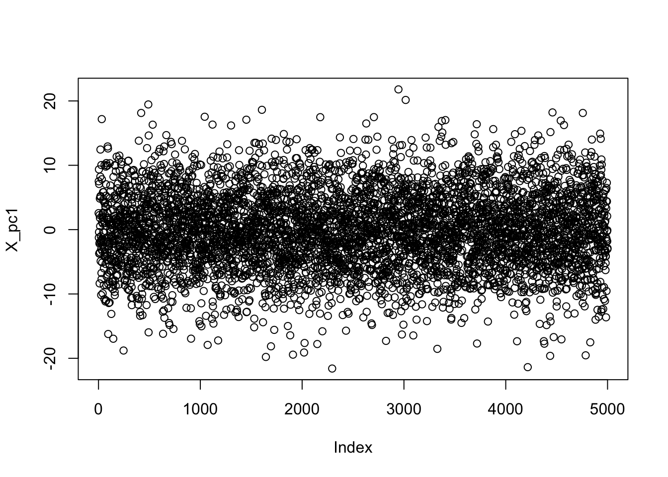

This was a situation where the rows were IID, so the ‘fuzzy caterpillar’ was not surprising. But let’s consider a pattern where there is structure to the rows, e.g., a multivariate time series.

Here I’m going to use the OpenMeteo website to pull temperature data from NYC, Boston, Philadelphia, Baltimore, and Washington DC for the past 6 months:

library(tidyverse)
library(httr2)
eps <- 0.2
cities <- tribble(
    ~city, ~lat, ~lon, 
    "NYC", 40.73, -73.93,
    "BOS", 42.36, -71.06,
    "PHL", 39.96, -75.17,
    "BAL", 39.29, -76.61,
    "WDC", 38.89, -77.03
) |> 
    mutate(lat_p = lat + eps, 
           lat_n = lat - eps, 
           lon_p = lon + eps, 
           lon_n = lon - eps)

resp <- request("https://api.open-meteo.com") |>
    req_url_path("v1/forecast") |>
    req_url_query(latitude=paste(cities$lat, collapse=","), 
                  longitude=paste(cities$lon, collapse=","),
                  hourly="temperature_2m", 
                  past_days=60) |>
    req_perform()

temperature_df <- resp |> 
    resp_body_json() |> 
    map(\(r) data.frame(time = r |> pluck("hourly", "time") |> list_c(), 
                        temperature_2m = r |> pluck("hourly", "temperature_2m") |> list_c(), 
                        latitude = r |> pluck("latitude"), 
                        longitude = r |> pluck("longitude"))) |> 
    list_rbind() |> 
    mutate(time=ymd_hm(time)) |> 
    left_join(cities, join_by(between(latitude, lat_n, lat_p), 
                              between(longitude, lon_n, lon_p))) |> 
    select(time, temperature_2m, city) |>
    pivot_wider(names_from=city, 
                values_from=temperature_2m) |>
    # Remove baseline temperature
    mutate(across(-time, \(x) x - mean(x))) 

glimpse(temperature_df)

Rows: 1,608
Columns: 6
$ time <dttm> 2026-03-07 00:00:00, 2026-03-07 01:00:00, 2026-03-07 02:00:00, 2…
$ NYC  <dbl> -7.946828, -8.146828, -8.246828, -8.346828, -8.446828, -8.446828,…
$ BOS  <dbl> -7.317724, -7.317724, -7.317724, -7.217724, -7.217724, -7.217724,…
$ PHL  <dbl> -7.888619, -8.288619, -8.588619, -8.888619, -9.088619, -9.288619,…
$ BAL  <dbl> -7.166667, -7.266667, -7.566667, -7.966667, -8.366667, -8.666667,…
$ WDC  <dbl> -6.31449, -6.61449, -6.91449, -7.21449, -7.61449, -8.01449, -8.71…

which gives us data like the following (except with 1608 rows):

	NYC	BOS	PHL	BAL	WDC
2026-03-07	-7.946828	-7.317724	-7.888619	-7.166667	-6.31449
2026-03-07 01:00:00	-8.146828	-7.317724	-8.288619	-7.266667	-6.61449
2026-03-07 02:00:00	-8.246828	-7.317724	-8.588619	-7.566667	-6.91449
2026-03-07 03:00:00	-8.346828	-7.217724	-8.888619	-7.966667	-7.21449
2026-03-07 04:00:00	-8.446828	-7.217724	-9.088619	-8.366667	-7.61449

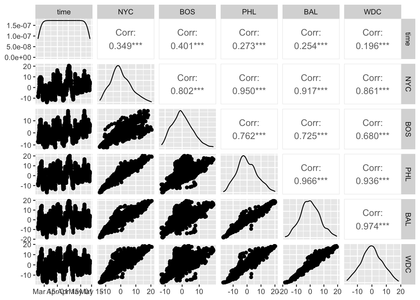
If we plot this, we can see a clear common temporal pattern with the day-night cycle:

library(GGally)
ggpairs(temperature_df)

So let’s now apply PCA to the temperature columns in this data set:

temperature_mat <- temperature_df |> 
  select(-time) |> 
  as.matrix()

temperature_pc1 <- pca_power_method(temperature_mat)

temperature_pc1 |> 
    pluck("v") |> 
    as.data.frame() |> 
    rownames_to_column("city") |> 
    inner_join(cities, join_by(city)) |> 
    arrange(desc(lat)) |> 
    mutate(city = factor(city, levels=city)) |> 
    ggplot(aes(x=city, y=V1)) + 
    geom_col(fill="#8B000033", color="red4") + 
    xlab("City") + 
    ylab("Principal Component 1") + 
    theme_bw()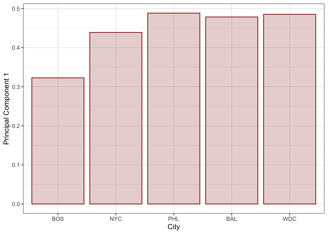

So we see that our PC takes a bit from each city, but is most heavily loaded on the southernmost cities in this sample.

If we return and look at \(\bX \bv_1\) or equivalently \(\bx_i^{\top}\bv_1\) for each observation \(i\), we get the following

temperature_mat %*% temperature_pc1$v |> 
  data.frame() |> 
  rename(pc_row=1) |> 
  mutate(time = temperature_df$time) |> 
  ggplot(aes(x=time, y=pc_row)) + 
  geom_point() + 
  xlab("Time") + 
  ylab("X * v")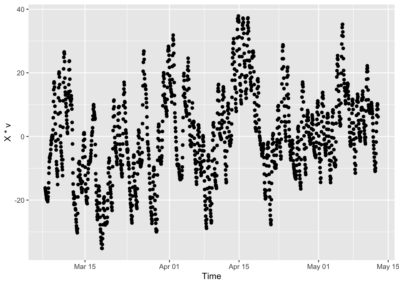

So there is a time structure! Note that this isn’t quite the time series we’d get from just an average of the five temperatures–it’s a weighted average via the columns above–but it’s close.

Let’s go ahead and add some cities from the other side of the world to get a more interesting pattern:

library(tidyverse)
library(httr2)
eps <- 0.2
cities <- tribble(
    ~city, ~lat, ~lon, 
    "NYC", 40.73, -73.93,
    "BOS", 42.36, -71.06,
    "PHL", 39.96, -75.17,
    "SYD", -33.87, 151.21,
    "MEL", -37.81, 144.97,
    "BNE", -27.47, 153.03
) |> 
    mutate(lat_p = lat + eps, 
           lat_n = lat - eps, 
           lon_p = lon + eps, 
           lon_n = lon - eps) 

resp <- request("https://api.open-meteo.com") |>
    req_url_path("v1/forecast") |>
    req_url_query(latitude=paste(cities$lat, collapse=","), 
                  longitude=paste(cities$lon, collapse=","),
                  hourly="temperature_2m", 
                  past_days=60) |>
    req_perform()

temperature_df2 <- resp |> 
    resp_body_json() |> 
    map(\(r) data.frame(time = r |> pluck("hourly", "time") |> list_c(), 
                        temperature_2m = r |> pluck("hourly", "temperature_2m") |> list_c(), 
                        latitude = r |> pluck("latitude"), 
                        longitude = r |> pluck("longitude"))) |> 
    list_rbind() |> 
    mutate(time=ymd_hm(time)) |> 
    left_join(cities, join_by(between(latitude, lat_n, lat_p), 
                              between(longitude, lon_n, lon_p))) |> 
    select(time, temperature_2m, city) |> 
    pivot_wider(names_from=city, 
                values_from=temperature_2m) |>
    mutate(across(-time, \(x) x - mean(x))) # Remove baseline temperature


temperature_mat2 <- temperature_df2 |> 
    select(-time) |> 
    as.matrix()

temperature2_pc1 <- pca_power_method(temperature_mat2)

temperature2_pc1 |> 
    pluck("v") |> 
    as.data.frame() |> 
    rownames_to_column("city") |> 
    inner_join(cities, join_by(city)) |> 
    arrange(desc(lat)) |> 
    mutate(city = factor(city, levels=city)) |> 
    ggplot(aes(x=city, y=V1)) + 
    geom_col(fill="#8B000033", color="red4") + 
    xlab("City") + 
    ylab("Principal Component 1") + 
    theme_bw()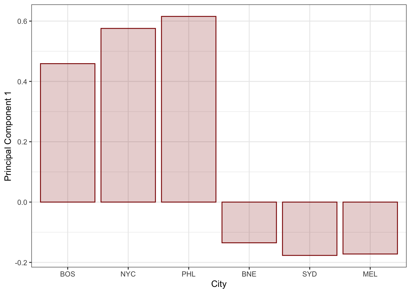

Here, we’ve augmented our US cities with the Australian cities of Sydney (SYD), Brisbane (BNE) and Melbourne (MEL). These cities are on the other side of the world from the US cities we’ve looked at and their temperatures move contrary to the US cities (both their seasonal cycles and their day-night cycles) so this isn’t too surprising.

Pause for Reflection

Modify the example above to include some Northern + Eastern Hemisphere cities like Beijing and Kyiv and some Southern + Western cities like Sao Paolo and Buenos Aires. What patterns do you find? Does this make sense? What does this tell you about weather patterns? What happens if you take daily average temperatures instead of hourly data?

As before, the ‘time series’ that goes with this data is interesting:

temperature_mat2 %*% temperature2_pc1$v |> 
  data.frame() |> 
  rename(pc_row=1) |> 
  mutate(time = temperature_df2$time) |> 
  ggplot(aes(x=time, y=pc_row)) + 
  geom_point() + 
  xlab("Time") + 
  ylab("X * v")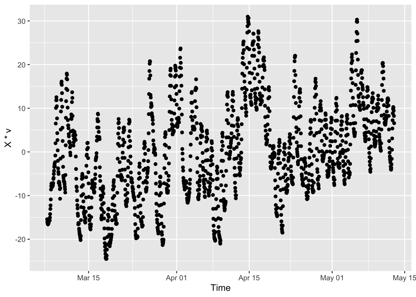

It’s actually not that different from what we saw above, in part because the time patterns are correlated. If we were to put these together, we would expect Sydney to move opposite this pattern (zigging when this pattern zags) since it has a negative loading.

A Singular Value Approach to PCA

Above, to get the time course, we computed \(\bX\bv\), but this is a bit hokey.

It’s easier to use the SVD-formulation of PCA, which we’ll now introduce. Given a matrix \(\bX \in \R^{n \times p}\), we want to break it up into a sum of simple components: for our purposes, these ‘simple’ components can be expressed as rank-1 matrices. That is, our ‘simple’ components are basically one-dimensional bits (line segments) in a higher-dimensional space. So we’re looking for something like:

\[\bX = \bX_1 + \bX_2 + \dots \]

If \(\bX\) is rank-\(k\), we should expect that we could use a sum of only \(k\) rank-1 terms to exactly equal \(\bX\). Determining the rank of a matrix is not trivial, but an upper bound is \(\text{rank}(\bX) \leq \min\{n, p\}\). That is, the rank of a matrix is bounded above by (and, it turns out, is typically equal to) its smaller dimension. So, if \(\bX \in \R^{3 \times 5}\), we know the rank of \(\bX\) - and hence the number of sum terms we will need - is at most 3. This shouldn’t surprise you - if we needed four degrees of freedom to reproduce 3 points, we would clearly be doing something inefficiently.

So we have our goal:

\[\bX = \bX_1 + \bX_2 + \dots + \bX_{\text{rank}(\bX)}\]

But these terms \(\bX_i\) are not so easy to work with. As noted above, the idea of forcing each \(\bX_i\) to be rank-1 is not easy, but we have a trick! Any rank-1 matrix can be written as the (outer) product of two vectors:

\[\bX_i = \bu_i\bv_i^{\top}\]

where \(\bu_i \in \R^n\) and \(\bv_i \in \R^p\). The fact that this gives a rank-1 term shouldn’t be too surprising: by going through two vectors, we essentially create a ‘bottleneck’ that forces things down to one dimension.

Obviously, this sort of \(\bu_i\bv_i^{\top}\) is not a unique representation of a given rank-1 matrix. If \(\bA\) were rank-1, we could write it as:

\[\bA = \bu \bv^{\top} = (\bu/2)(2\bv)^{\top} = (\alpha\bu)(\bv/\alpha)^{\top} \text{ for any } \alpha \neq 0\]

To avoid this, let’s force \(\bu\) and \(\bv\) to be unit vectors and to put any scale factors outside the product: so, we would have something like

\[\bA = d\, \bu\bv^{\top}\]

where \(d\) is a scalar and \(\bu \in \R^n, \bv \in \R^p\) are unit vectors. We still have a bit of sign ambiguity (\(d\bu = (-d)(-\bu)\)) but we can fix this by setting \(d > 0\).³

So now, we know we want to break up our original data matrix \(\bX\) as:

\[\bX = d_1\bu_1\bv_1^{\top} + d_2\bu_2\bv_2^{\top} + \dots d_k\bu_k\bv_k^{\top}\]

where \(k = \text{rank}(\bX)\). This seems so much harder! But we have a trick up our sleeves.

Think back to when we introduced the singular value decomposition of a matrix \(\bX\). Recall that we had

\[\bX = \bU\bD\bV^{\top}\]

where

\(\bD\) is a diagonal matrix with all positive elements on the diagonal
\(\bU\) and \(\bV\) are an orthogonal matrices

At the time, I said not to be too concerned about the exact dimensions of each term, but we can now be precise:

\[\bX = \bU\bD\bV^{\top}\]

for a rank-\(k\) matrix where

\(\bD \in \R^{k \times k}\) is a diagonal matrix with all positive values on the diagonal
\(\bU \in \R^{n \times k}\) is an orthogonal matrix satisfying \(\bU^{\top}\bU = \bI_{k \times k}\)
\(\bV \in \R^{p \times k}\) is an orthogonal matrix satisfying \(\bV^{\top}\bV = \bI_{k \times k}\)

With this precise definition in place, let’s start to expand this sum out. Because \(\bD\) is diagonal, we see that:

\[\begin{align*} \bX &= \bU\bD\bV^{\top} \\ &= \begin{pmatrix} \bu_1 \\ \bu_2 \\ \dots \\ \bu_k \end{pmatrix} \begin{pmatrix} d_1 \\ 0 & d_2 \\ && \ddots \\ &&& d_k \end{pmatrix} \begin{pmatrix} \bv_1 \\ \bv_2 \\ \dots \\ \bv_k \end{pmatrix}^{\top} \\ &= \begin{pmatrix} d_1\bu_1 \\ d_2\bu_2 \\ \dots \\ d_k\bu_k \end{pmatrix} \begin{pmatrix} \bv_1 \\ \bv_2 \\ \dots \\ \bv_k \end{pmatrix}^{\top} \\ &= d_1\bu_1\bv_1^{\top} + d_2\bu_2\bv_2^{\top} + \dots + d_k\bu_k\bv_k^{\top} \end{align*}\]

So the SVD gives us exactly the PCA decomposition we were looking for. If you look inside most PCA software (e.g., sklearn.PCA in Python or stats::prcomp in R), you will see that it’s all just really a wrapper around an SVD.

In fact, let’s just go ahead and use an SVD to do PCA ‘by hand’:

temp_svd <- svd(temperature_mat2)
temp_u1 <- temp_svd$u[,1]
temp_v1 <- temp_svd$v[,1]

library(patchwork)
p1 <- data.frame(u = temp_u1, time=temperature_df2$time) |>
  ggplot(aes(x=time, y=u)) + 
  geom_line() + 
  geom_point(alpha=0.2) + 
  xlab("Time Axis") + 
  ylab("U-Factor from PC1") + 
  theme_bw()

p2 <- data.frame(v = temp_v1, city=cities$city) |>
  ggplot(aes(x=city, y=v)) + 
  geom_col() + 
  geom_point() + 
  xlab("City") + 
  ylab("V-Factor from PC1") + 
  theme_bw()

p1 / p2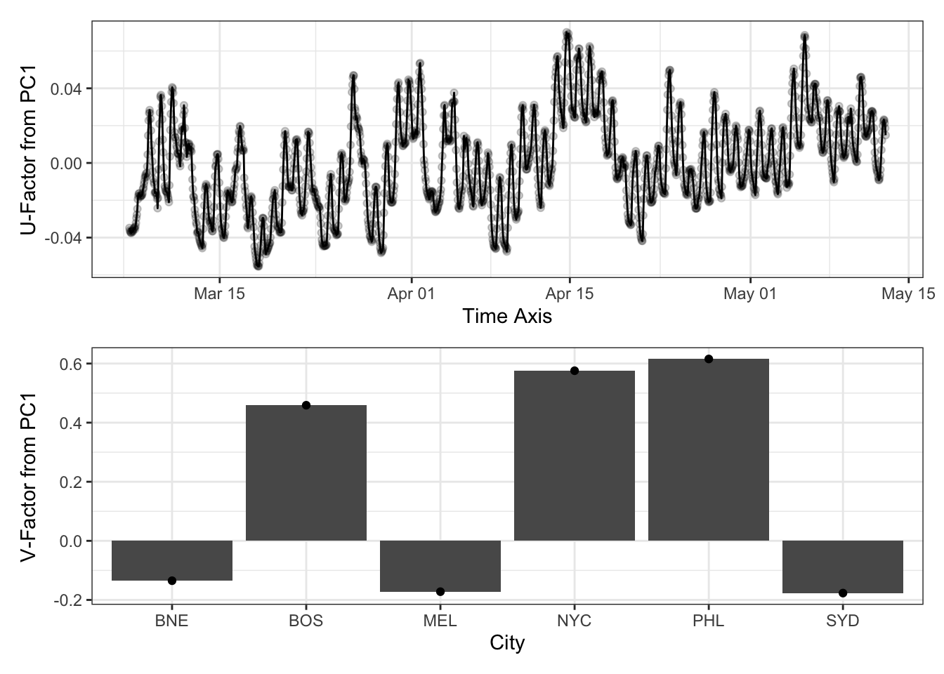

This is (up to scaling - via that \(d\) term) what we saw before!

So the svd() gets us everything we want, but it’s a bit magic. We can also ‘build-our-own’ SVD by returning to our approximation problem. To get the first PC, we can write the problem of approximating \(\bX\) as:

\[\argmin_{d, \bu, \bv} \|\bX - d\bu\bv^{\top}\|_2^2\]

Here, we want to pick \(d, \bu, \bv\) to approximate \(\bX\) as well as possible. After a bit of algebra, we can show this becomes

\[\argmax_{\bu, \bv} \bu^{\top}\bX\bv\]

Deriving the SVD Approximation Problem

We begin with

\[\argmin_{d, \bu, \bv} \|\bX - d\bu\bv^{\top}\|_2^2\]

If we expand out the binomial, this becomes:

\[\begin{align*} \|\bX - d\bu\bv^{\top}\|_2^2 &= \Tr\left[(\bX - d\bu\bv^{\top})^{\top}(\bX - d\bu\bv^{\top})\right] \\ &= \Tr\left[(\bX^{\top} - d\bv\bu^{\top})(\bX - d\bu\bv^{\top})\right] \\ &= \Tr\left[\bX^{\top}\bX- d\bv\bu^{\top}\bX - d\bX^{\top}\bu\bv^{\top} + d^2\bv\bu^{\top}\bu\bv^{\top}\right] \\ &= \|\bX\|_2^2 - d\Tr(\bv\bu^{\top}\bX) - d\Tr(\bX^{\top}\bu\bv^{\top}) + d^2\Tr(\bv\bu^{\top}\bu\bv^{\top}) \\ &= \|\bX\|_2^2 - d\Tr(\bu^{\top}\bX\bv) - d\Tr(\bv^{\top}\bX^{\top}\bu) + d^2\Tr(\bv\|\bu\|_2^2\bv^{\top}) \\ &= \|\bX\|_2^2 - d\Tr(\bu^{\top}\bX\bv) - d\Tr(\bu^{\top}\bX\bv) + d^2\Tr(\bv^{\top}\bv) \\ &= \|\bX\|_2^2 - 2d\Tr(\bu^{\top}\bX\bv) + d^2 \\ &= \|\bX\|_2^2 - 2d(\bu^{\top}\bX\bv) + d^2 \end{align*}\]

Holding off on finding \(\bu, \bv\) for now, let’s find an optimal \(d\). As always, let’s take the derivative with respect to \(d\) and set it to zero:

\[ 0 = -2(\bu^{\top}\bX\bv) + 2d \implies d = \bu^{\top}\bX\bv\]

Putting this into above, we have an objective of:

\[\begin{align*} \argmin_{\bu, \bv} \|\bX\|_2^2 - 2d(\bu^{\top}\bX\bv) + d^2 &= \argmin_{\bu, \bv} \|\bX\|_2^2 - (\bu^{\top}\bX\bv)^2 \end{align*}\]

From here, we note that \(\bX\) is unchanging - it’s the data we’re trying to approximate - so we really just have

\[ \argmin_{\bu, \bv} - (\bu^{\top}\bX\bv)^2\]

which we can rewrite as

\[ \argmax_{\bu, \bv} \bu^{\top}\bX\bv \]

So what does this problem really mean? We’re looking for \(\bu, \bv\) that maximize this term. Informally, you can think of this as finding the \(\bu, \bv\) that are best aligned with \(\bX\). A bit more rigorously, if we expand \(\bX\) out with its SVD:

\[\begin{align*} \argmax_{\bu\bv} \bu^{\top}\bX\bv &= \argmax_{\bu\bv} \bu^{\top}\left(\sum d_i \bu_i\bv_i^{\top}\right)\bv \\ &= \argmax_{\bu\bv} \sum d_i (\bu^{\top}\bu_i)(\bv_i^{\top}\bv \end{align*}\]

So our objective is some weighted combination of the \(d_i\) values, based on how aligned our \(\bu\) is with each ‘real’ \(\bu_i\). Since the \(d_i\) are ordered, the best solution is the one we get when \(\bu = \bu_1\) and \(\bv = \bv_1\), which is exactly what we want!

So now that we’ve convinced ourselves that

\[\argmax_{\substack{\bu \in \R^n, \bv \in \R^p \\ \|\bu\| = \|\bv\|=1}} \bu^{\top}\bX\bv\]

is the problem we want to solve, how do we actually do that? We have two variables and handling them both at the same time is tricky, so let’s just do one at a time. If we fix \(\bv\), it’s easy to see that the best \(\bu\) is the one that is just aligned with \(\bX\bv\); similarly, if we fix \(\bu\), the best \(\bv\) is just one aligned with \(\bu^{\top}\bX\). We can put these together into an power method algorithm that looks similar to the one we developed above for just \(\bv\):

Initialize \(\bv^{(0)}\) randomly
Repeat the following until convergence: \[ \bu^{(k)} \leftarrow \frac{\bX\bv^{(k)}}{\|\bX\bv^{(k)}\|}\] \[ \bv^{(k+1)} \leftarrow \frac{\bX^{\top}\bu^{(k)}}{\|\bX^{\top}\bu^{(k)}\|}\]

In code, this might look something like:

pca_power_svd <- function(X, thresh=1e-8){
    n <- NROW(X); p <- NCOL(X)
    
    normalize <- function(x) x / sqrt(sum(x^2))
    
    v <- normalize(matrix(rnorm(p), ncol=1))
    
    repeat {
        u <- normalize(X %*% v)
      
        v_old <- v
        v <- normalize(t(X) %*% u)
        
        # To fix sign irregularity, force v[1] > 0
        if(v[1] < 0) v <- -v
        
        if(sum(abs(v - v_old)) < thresh){
            break
        }
    }
    
    list(u=u, v=v, d=t(u) %*% X %*% v)
}

which gives us:

pca_svd_temp <- pca_power_svd(temperature_mat2)

p1 <- data.frame(u=pca_svd_temp$u, time=temperature_df2$time) |>
  ggplot(aes(x=time, y=u)) + 
  geom_line() + 
  geom_point(alpha=0.2) + 
  xlab("Time Axis") + 
  ylab("U-Factor from PC1") + 
  theme_bw()

p2 <- data.frame(v=pca_svd_temp$v, city=cities$city) |>
  ggplot(aes(x=city, y=v)) + 
  geom_col() + 
  geom_point() + 
  xlab("City") + 
  ylab("V-Factor from PC1") + 
  theme_bw()

p1 / p2

which matches what we got doing it with the built-in svd().

Making Sense of PCA

The temperature results above are interesting, but not the easiest to interpret. Australia being ‘opposite’ the US makes sense, but if we want to go deeper in our analysis, what should we do? I like the strategy of using PCs to build an ‘estimated’ \(\bX\), based on the ‘sum of simple’ components above. In the easiest case, we can make sense the first PC by looking into

\[\hat{\bX}_1 = d_1 \bu_1 \bv_1^{\top} \in \R^{n \times p}\]

Regularized PCA

Other Applications of PCA-Type Decompositions

Footnotes

Later, we will use a more generalized notion of ‘dimension’, leading us to the task of manifold learning.↩︎
A matrix of size \(p \times p\) can have up to \(p\) eigenvalue-eigenvector pairs. Because we are maximizing \(\bv^{\top}\bX^{\top}\bX\bv\), we want the maximal (or leading) eigenvector-eigenvalue pair, defined as the one for which the (absolute value of) the eigenvalue is the largest.↩︎
You might still notice we have a \(\bu\bv^{\top} = (-\bu)(-\bv)^{\top}\) ambiguity. This actually can’t be resolved uniquely and is a bit beyond our course, but most software will typically do something meaningless like “make the first value of \(\bu\) positive” or “make the largest value of \(\bu\) positive.”↩︎