STA 9890 - Spring 2025
Test 3: Unsupervised Learning

The original test booklet can be found here. \[\newcommand{\bX}{\mathbf{X}}\newcommand{\by}{\mathbf{y}}\newcommand{\bx}{\mathbf{x}}\newcommand{\R}{\mathbb{R}}\newcommand{\N}{\mathbb{N}}\newcommand{\bbeta}{\mathbf{\beta}}\newcommand{\argmin}{\text{arg min}}\newcommand{\bD}{\mathbf{D}}\newcommand{\bzero}{\mathbf{0}}\newcommand{\bI}{\mathbf{I}}\newcommand{\bz}{\mathbf{z}} \newcommand{\P}{\mathbb{P}}\]

Multiple Choice (30 points - 10 questions at 3 points each)

True/False: PCA cannot be applied without centering the data first.

Solution

False - PCA can be applied without centering the data first if your primary goal is to understand the mean structure of complex and high-dimensional data. The second PC will then be the first PC of the covariance after fitting a particular low-rank mean model

True/False: The singular values of a (real-valued) matrix are always positive.

Solution

True. In fact, it is not even required that the matrix be real-valued: complex-valued matrices have real singular values as well (since singular values capture the magnitude of the ‘stretch’ in a certain direction). To wit,

n <- 4
p <- 3
X <- matrix(complex(real=rnorm(n * p), 
                    imaginary=rnorm(n * p)), 
            nrow=n)
D <- diag(svd(X)$d)
U <- svd(X)$u
V <- svd(X)$v

D

         [,1]     [,2]      [,3]
[1,] 3.603399 0.000000 0.0000000
[2,] 0.000000 2.560264 0.0000000
[3,] 0.000000 0.000000 0.5576813

This satisfies the ‘standard’ SVD structure, if we use the conjugate transpose of $\bV$ instead of the regular transpose.

all.equal(X, U %*% D %*% t(Conj(V)))

[1] TRUE

The $\bU$, $\bV$ matrices are now Hermitian (not orthogonal) matrices and satisfy $\bU^{H}\bU = \bI$ and $\bV^{H}\bV = \bI$ instead:

h <- function(x) t(Conj(x))
zapsmall(h(U) %*% U)

     [,1] [,2] [,3]
[1,] 1+0i 0+0i 0+0i
[2,] 0+0i 1+0i 0+0i
[3,] 0+0i 0+0i 1+0i

and

zapsmall(h(V) %*% V)

     [,1] [,2] [,3]
[1,] 1+0i 0+0i 0+0i
[2,] 0+0i 1+0i 0+0i
[3,] 0+0i 0+0i 1+0i

Estimated principal components are orthogonal to the data.

Solution

False. PCs are not orthogonal to the data: they are in fact, ‘optimally correlated’ with the data to capture as much variance as possible.

PCs are generally orthogonal with each other and with the residual (deflated) data, though this assumption may be relaxed for certain versions of Sparse PCA. See this paper for details
The sample covariance matrix of a data set is always strictly positive definite (all eigenvalues strictly greater than zero).
Solution
False. Oh that it were so!

The rank (number of non-zero eigenvalues) of a covariance matrix estimated from a data matrix of size $n$-$times$-$p$ is at most $\min\{n, p\}$, so in the high-dimensional context, we don’t have enough ($p$) non-zero.

To wit:
n <- 5 p <- 50 X <- matrix(rnorm(n * p), nrow=n) # Computing this numerically, there's a bit of 'trash' # we need to discard sum(eigen(crossprod(X))$values > 1e-8)

[1] 5
Equivalently (and more directly):
svd(X)$d

[1] 8.360675 7.854200 7.295551 6.591210 4.920648
To address this problem, there is a large literature on high-dimensional covariance estimation. While we do not focus on high-dimensional covariance estimation in this class, it is quite a rich subject: if you want dig further into it, the Ledoit-Wolf estimator is a good place to start.
Select One: Which of the following relates the singular values of $\bX$ ($\sigma_i$) and the eigenvalues of $\bX^{\top}\bX$ ($\lambda_i$) for all $i = 1, \dots, \textsf{Rank}(\bX)$?
- $\sigma_i=\lambda_i$
- $\sigma_i^2 = \lambda_i$
- $\sigma_i = \lambda_i^2$
- $\sigma_i \geq \lambda_i$
- $\sigma_i \leq \lambda_i$
Solution

The correct relation is $\sigma_i^2 = \lambda_i$. (Note that one or both of the inequalities may be true depending on $\sigma_i \geq 1$ or $\sigma_i \leq 1$ but they do not hold universally.)

To see this, let

\[\bX = \bU\bD\bV^{\top} \implies \bX^{\top}\bX = (\bU\bD\bV^{\top})^{\top}(\bU\bD\bV^{\top}) = \bV\bD^2\bV^{\top}\]

so the eigenvalues (found in $\bD^2$) are the squares of the singular values (found in $\bD$).
Select One: Which of the following is not a common rule for selecting the PCA rank?
- Elbow Rule
- 80% Rule
- Boulder Plot
- Hypothesis Testing
Solution

The Boulder Plot is not a common method of PCA rank selection. (The name, designed to be a red herring, is an oblique reference to the scree or elbow plot, but the point of the scree plot is that there aren’t major components ‘boulders’ beyond the curve.)
Select One: Which of the following pairs of vectors are orthogonal?
- Loading Vector $i$ and Loading Vector $i+2$
- Score Vector $j$ and Score Vector $j-1$
- Loading Vector $k$ and Score Vector $k+1$
Solution

There is no orthogonality relationship per se between loading and score vectors. In fact, the loading and score vectors live in different spaces ($\R^n$ vs $\R^p$) so there isn’t even an appropriate inner product for them to be orthogonal under.
Select All That Apply: Which of the following are properties of (generic/standard) PCA decomposition?
- Additive
- Ordered
- Orthogonal
- Regularized
- Sparse
- Non-Negative
- Nested
- Easily-Computed to Global Optimality
- Convex
Solution
- ✅ Additive
- ✅ Ordered
- ✅ Orthogonal
- Regularized
- Sparse
- Non-Negative
- ✅ Nested
- ✅ Easily-Computed to Global Optimality
- Convex
Select All That Apply: Which of the following are properties of Non-Negative Matrix Factorization?
- Additive
- Ordered
- Orthogonal
- Regularized
- Sparse
- Non-Negative
- Nested
- Easily-Computed to Global Optimality
- Convex
Solution
- ✅ Additive
- Ordered
- Orthogonal
- ✅ Regularized
- ✅ Sparse
- ✅ Non-Negative
- Nested
- Easily-Computed to Global Optimality
- Convex
Most NMF variants are non-convex, but at least one well known convex variant exists, so I will accept that answer. I will accept “easily-computed” iff you select convex.
Select All That Apply: Which of the following are properties of sparse PCA decomposition?
- Additive
- Ordered
- Orthogonal
- Regularized
- Sparse
- Non-Negative
- Nested
- Easily-Computed to Global Optimality
- Convex
Solution
- ✅ Additive
- ✅ Ordered
- Orthogonal
- ✅ Regularized
- ✅ Sparse
- Non-Negative
- ✅ Nested
- Easily-Computed to Global Optimality
- Convex
Most sparse PCA variants are not orthogonal, but certain orthogonal variants have been proposed relying on rather tricky optimization, so I will allow that answer.

Similarly, most sparse PCA is non-convex, but certain convex relaxations have been proposed so I will allow that answer. I will allow easily computed iff you select convex.

Mathematics of Machine Learning (20 Points Total)

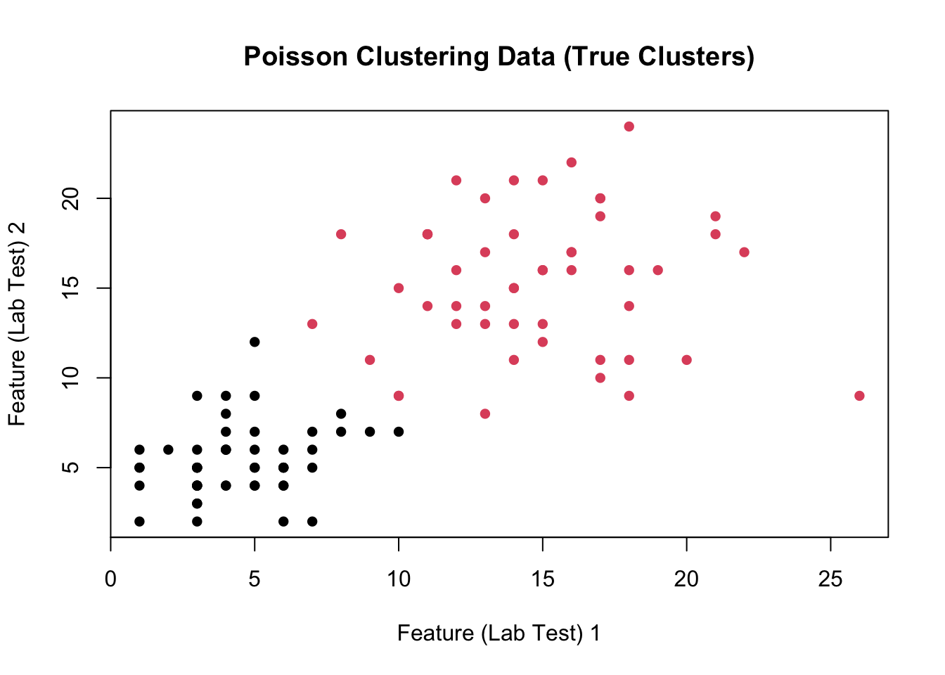
In this problem, you will derive a $K$-Means-type clustering algorithm for bivariate Poisson data. Specifically, you will use the EM-Framework to cluster data that is generated from the following statistical model:

For each data point, $\bx \in \N^2$, both coordinates $(x^{(1)}, x^{(2)})$ are sampled IID from a Poisson distribution with (common) mean $\lambda$. The value of $\lambda$ depends on the underlying (but unknown) class: formally,

\[\bx_i | i \in \text{Cluster-$j$} \buildrel{\text{iid}}\over\sim \text{Poisson}^{\otimes 2}(\lambda_j)\]

You can think of this is a model for clustering genetic data where $i$ indexes patients, $j$ indexes disease subtypes, and each patient has their gene expression values processed by two different IID labs for reliability.

Recall that the Poisson distribution with parameter $\lambda$ has a PMF given by:

\[\P(X = x) = \frac{\lambda^x e^{-\lambda}}{x!}\]

M-Step: To build the M-Step of our clustering algorithm, we need to determine the maximum likelihood estimator (MLE) of the Poisson parameters $\lambda_j$. Recall that, within a cluster, our data are IID so we will begin by deriving the MLE for IID Poisson samples. (10 points total)
1. Suppose a single point $z$ is observed from a Poisson distribution with unknown parameter $\theta$. What is the negative log-likelihood associated with this observation? (2 points)
  
  Recall: The likelihood is a function of the parameter, $\theta$, holding the data $z$ constant.
  
  Solution
  
  If the PMF is $f_{\lambda}(z) = \lambda^z e^{-\lambda} / z!$, the loglikelihood is obtained by making $\lambda$ the argument and taking logs to get
  
  \[\begin{align*} f_{\lambda}(z) &= \lambda^z e^{-\lambda} / z! \\ \log f_{\lambda}(z) &= z \log(\lambda) - \lambda - \log(z!)\\ \ell(\lambda) &= z \log(\lambda) - \lambda - \log(z!) \end{align*}\]
2. Now, suppose we have $n$ IID samples ($z_1, z_2, \dots, z_n$) from the same distribution. What is the joint negative log-likelihood associated with these observations? (3 points)
  
  Solution
  
  Because PMFs of independent samples multiply, their NLL adds:
  
  \[\begin{align*} \ell(\lambda; z) &= z \log(\lambda) - \lambda - \log(z!) \\ \implies \ell(\lambda; \{z_1, z_2, \dots, z_n\}) &= \sum_{i=1}^n \ell(\lambda; z_i) \\ &= \sum_{i=1}^n z_i \log(\lambda) - \lambda - \log(z_i!)\\ &= -n \lambda + \sum_{i=1}^n z_i \log(\lambda) - \log(z_i!)\\ &= -n \lambda + \log(\lambda) \sum_{i=1}^n z_i- \log(z_i!) \end{align*}\]
  
  or equivalent.
3. What is the maximum likelihood estimator associated with this observation? Recall that the MLE is the value of the parameter that maximizes the likelihood, or equivalently maximizes the log-likelihood (or equivalently minimizes the negative log-likelihood) (3 points)
  
  Solution
  
  Taking the gradient of the above with respect to $\lambda$, we find the MLE is:
  
  \[\begin{align*} 0 &= \frac{\text{d}\,\ell(\lambda)}{\text{d}\,\lambda} \\ &= \frac{\text{d}\,}{\text{d}\,\lambda}\left[-n \lambda + \log(\lambda)\sum_{i=1}^n -z_i + \log(z_i!)\right] \\ &= -n + \lambda^{-1}\sum_{i=1}^n z_i + 0 \\ n &= \lambda^{-1} \sum_{i=1}^n z_i \\ \implies \hat{\lambda}_{\text{MLE}} &= \frac{\sum_{i=1}^n z_i}{n} \end{align*}\]
  
  So the MLE for the mean parameter $\lambda$ is just the sample mean. (This is not always the case, but the Poisson is a member of a nice family of distributions where these types of calculations often have nice interpretations.)
4. For our bivariate model, we have multiple data values $z_i^{(1)}, z_i^{(2)}$ for each observation instead. How should we modify our MLE for this data? What is the resulting MLE? (2 points)
  
  Recall that the two values per observation are IID.
  
  Solution
  
  Because the data can essentially be treated as a ‘double sample’, the MLE is simply
  
  \[\hat{\lambda}_{\text{MLE}} &= \frac{\sum_{i=1}^n x_i^{(1)} + x_i^{(2)}}{2n}\]
E-Step: To build the E-Step of our clustering algorithm, we need a rule for guessing the most probable class label for each observation. That is, assuming we know $\lambda_1, \lambda_2, \dots, \lambda_K$, we build a classification rule for each observation $\bx_i$. For this analysis, we will fix $K=2$. (5 points total)
1. Given a new observation $\bx_i$, compute its PMF under class $1$ ($\lambda = \lambda_1$) and class $2$ ($\lambda = \lambda_2$). (2 points)
  
  Solution
  
  Given $\bx$, our PMFs for class 1 and class 2 are
  
  \[\P_i(\bx) = \P_i(x^{(1)})\P_i(x^{(2)}) = \frac{\lambda_i^{x^{(1)}}e^{-\lambda_i}}{x^{(1)}!}\frac{\lambda_i^{x^{(2)}}e^{-\lambda_i}}{x^{(2)}!}=\frac{\lambda_i^{x^{(1)} + x^{(2)}} e^{-2\lambda_i}}{x^{(1)}!x^{(2)}!} \text{ for } i = 1, 2\]
2. Determine the relevant classification rule as a (simple) function of $x^{(1)}_i, x^{(2)}_i, \lambda_1, \lambda_2$.
  
  You may assume (without loss of generality) that $\lambda_1 > \lambda_2$. (3 points)
  Solution
  We will classify to the most likely class, so we can look at the PMF ratio:
  
  \[\begin{align*} \frac{\P_1(\bx)}{\P_2(\bx)} &= \frac{\frac{\lambda_1^{x^{(1)} + x^{(2)}} e^{-2\lambda_1}}{x^{(1)}!x^{(2)}!}}{\frac{\lambda_2^{x^{(1)} + x^{(2)}} e^{-2\lambda_2}}{x^{(1)}!x^{(2)}!}} \\ &= \left(\frac{\lambda_1}{\lambda_2}\right)^{x^{(1)} + x^{(2)}} e^{2(\lambda_2 - \lambda_1)} \end{align*}\]
  
  Since our decision is class 1 at values where this ratio is greater than 1, we can simply find the conditions on $\bx$ where its logarithm is greater than zero:
  
  \[\begin{align*} \log \frac{\P_1(\bx)}{\P_2(\bx)} &= (x^{(1)} + x^{(2)}) \log(\lambda_1 / \lambda_2) + 2(\lambda_2 - \lambda_1) \\ &= \frac{(x^{(1)} + x^{(2)})}{2} \log(\lambda_1 / \lambda_2) + (\lambda_2 - \lambda_1) \\ 0 & \leq \frac{(x^{(1)} + x^{(2)})}{2} \log(\lambda_1 / \lambda_2) + (\lambda_2 - \lambda_1)\\ \lambda_1 - \lambda_2 &\leq \frac{(x^{(1)} + x^{(2)})}{2} \log(\lambda_1 / \lambda_2) \\ \implies \frac{x^{(1)} + x^{(2)}}{2} &\geq \frac{\lambda_1-\lambda_2}{\log(\lambda_1) - \log(\lambda_2)} \end{align*}\]
  
  so we classify to $\lambda_1$ if the average of the two observations is greater than the quantity \[\frac{\lambda_1 - \lambda_2}{\log(\lambda_1) - \log(\lambda_2)}.\]
  
  I don’t have an intuitive way to derive or explain this formula, but we can verify that it indeed works.
  
  lambda_1 <- 5 lambda_2 <- 3 x <- rpois(2, lambda=lambda_1) sum(log(dpois(x, lambda=lambda_1))) > sum(log(dpois(x, lambda=lambda_2)))
  
  [1] TRUE
  
  vs
  
  mean(x) > (lambda_1 - lambda_2) / (log(lambda_1) - log(lambda_2))
  
  [1] TRUE

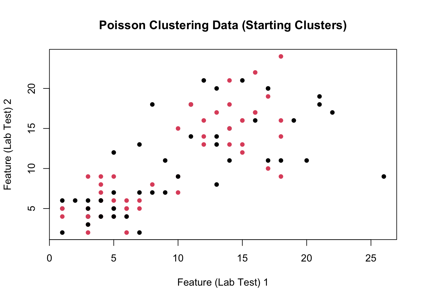
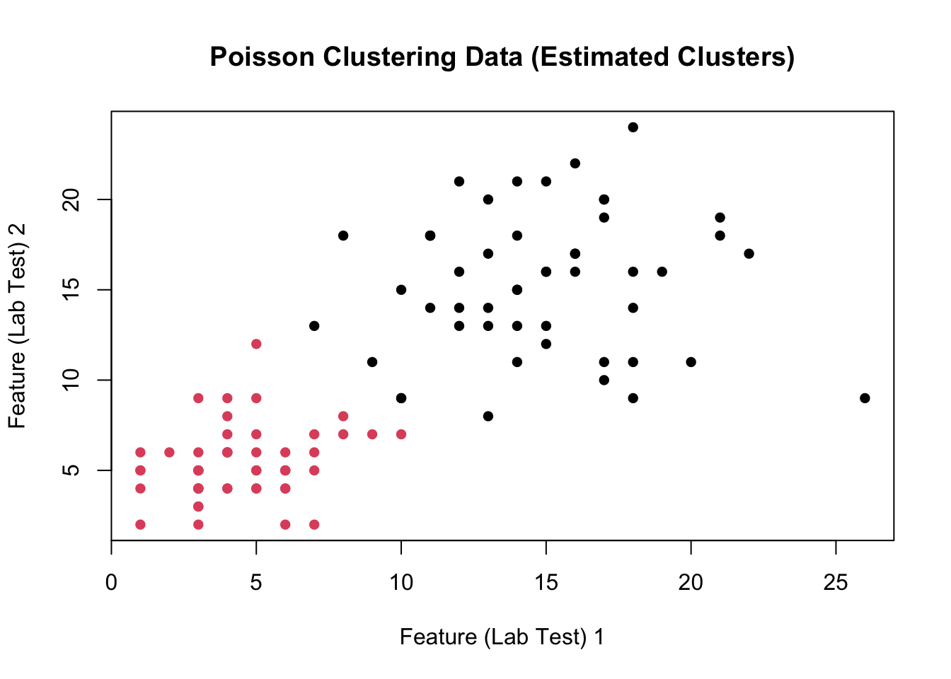
Finally, we are ready to put these steps together into a single unified clustering algorithm. Fill out the skeleton below using the M- and E-Steps you derived above (5 points)

Solution

Input: $n$ samples: $\bx_1, \bx_2, \dots, \bx_n$
Initialize: Set labels randomly $C_1 = \begin{cases} 1 & \text{ with probability } 0.5 \\ 2 & \text{ otherwise } \end{cases} \text{ for } i = 1,\dots,n$
Repeat:
- M-Step: For $k=1, 2$: update clusters \[\hat{\lambda}_k = \frac{1}{|\{i: C_i = k\}}\sum_{i: C_i = k} x^{(1)}_i + x^{(2)}_i\]
- E-Step: For $i=1, \dots, n$, reset labels: \[C_i = \begin{cases} 1 & \text{ if } \frac{x_i^{(1)} + x^{(2)}_i}{2} > \frac{\lambda_1-\lambda_2}{\log(\lambda_1) - \log(\lambda_2)} \\ 2 & \text{ otherwise } \end{cases}\]
Until: the labels ($\{C_i\}_{i=1}^n$) do not change between iterations or the maximum number of iterations has been reached
Return: Estimated Labels

Additional Details

We can implement this rather simply in R:

set.seed(100)
n <- 50

lambda_1 <- 5
lambda_2 <- 15

X <- matrix(rpois(4 * n, lambda=c(lambda_1, lambda_2)),
            nrow=2 * n, byrow=FALSE)

 true_labels <- rep(c(1, 2), times=50)

plot(X[,1], X[,2], col=true_labels, pch=16, 
     xlab="Feature (Lab Test) 1", 
     ylab="Feature (Lab Test) 2", 
     main="Poisson Clustering Data (True Clusters)"
     )

Applying our algorithm:

starting_labels <- sample(c(1, 2), size=NROW(X), prob=c(0.5, 0.5), replace=TRUE)

plot(X[,1], X[,2], col=starting_labels, pch=16, 
     xlab="Feature (Lab Test) 1", 
     ylab="Feature (Lab Test) 2", 
     main="Poisson Clustering Data (Starting Clusters)"
     )

which our algorithm improves to:

labels <- starting_labels
repeat {
   old_labels <- labels

   # Update centroids - M Step
   lambda_1_hat <- mean(X[labels == 1,])
   lambda_2_hat <- mean(X[labels == 2,])

   # Update labels - E Step
   X1 <- X[,1]; X2 <- X[,2]
   thresh <- (lambda_1_hat - lambda_2_hat) / log(lambda_1_hat / lambda_2_hat)
   labels = ifelse((X1 + X2)/2 > thresh, 1, 2)

   if(all(labels == old_labels)) break
}

print(labels)

  [1] 2 1 2 1 2 1 2 1 2 1 2 1 2 1 2 1 2 1 2 1 2 1 2 1 2 1 2 1 2 1 2 1 2 1 2 1 2
 [38] 1 2 1 2 1 2 1 2 1 2 1 2 1 2 1 2 1 2 1 2 1 2 1 2 1 2 1 2 1 2 1 2 1 2 1 2 1
 [75] 2 1 2 1 2 1 2 1 2 1 2 1 2 1 2 1 2 1 2 1 2 1 2 1 2 1

plot(X[,1], X[,2], col=labels, pch=16, 
     xlab="Feature (Lab Test) 1", 
     ylab="Feature (Lab Test) 2", 
     main="Poisson Clustering Data (Estimated Clusters)"
     )

which looks pretty good!

Numerically,

ARI <- mclust::adjustedRandIndex

ARI(labels, rep(c(1,2), times=50))

[1] 1

which exceeds (by just a bit) what we’d get from standard (Gaussian) $K$-Means:

kmeans_fit <- kmeans(X, centers=2)

ARI(kmeans_fit$cluster, true_labels)

[1] 0.8448428

We can verify that this isn’t purely just an artifact of poor initialization:

kmeans_fit <- kmeans(X, centers=2, nstart=500)

ARI(kmeans_fit$cluster, true_labels)

[1] 0.8448428

In fact, $K$-means gets a worse answer even when we give it the ‘true’ cluster centers as a starting point:

oracle_centers <- matrix(c(lambda_1, lambda_1, 
                           lambda_2, lambda_2), 
                         nrow=2, byrow=TRUE)
oracle_kmeans_fit <- kmeans(X, centers=oracle_centers)

ARI(oracle_kmeans_fit$cluster, true_labels)

[1] 0.8448428

For this very simple model, the difference really comes from the fact that:

We have a Poisson specific decision rule
We estimate one mean for both coordinates as opposed to a different mean for the $x, y$ coordinates.

Neither of these are huge changes, but hopefully you can see how this principle of model-based clustering can be usefully applied more broadly.

Practice of ML - Supervised (25 points total)

In this issue spotter question, I will describe a theoretical application of supervised machine learning. As described, this application falls short of “best practices” in several regards. Identify five places where this pipeline could be improved and recommend alternative (superior) practices. For each issue, you will receive:

1 point for identifying a valid issue
(Up to) 2 points for explaining what is wrong with the described practice and what impact / bias / error would be induced
(Up to) 2 points for accurately describing an alternative approach

Scenario:

You have been hired to build a extreme weather prediction system for the City of New York. For the first stage of your project, the client has asked you to focus on predicting periods of extreme rainfall.

To train your model, you have collected hourly rainfall data for the previous 25 years, giving a total of $n=219,250$ training points. With each training point, you have also collected several predictors from weather stations surrounding NYC:

Temperature

Time of Day

Wind speed

Wind direction

Cloud cover percentage

Relative Humidity

Barometric Pressure

Visibility

Rate of Precipitation

You have each of these measured contemporaneously, at one hour lag, at a three hour lag, and at a 24 hour lag, giving a total of $p=36$ features.

Given the dimensions of your data, you prefer to use a linear model and you begin by fitting a ridge regression model to all $n=219,250$ training points. You observe an error of approximately $0.5$ inches RMSE. In order to make your model more interpretable, you fit a lasso model. In order to tune $\lambda$, you pick $\lambda$ so that your MSE matches that which you got from ridge regression. This gives you a model with 5 important features. Because the difference between “extreme” rain and “average” rain is more than 0.5in, you consider your model to be sufficiently accurate to deliver to the customer.

After you send your results to your customer, your boss calls you into the office and provides some “rather emphatic” feedback. Based on this feedback, you scrap your model building process and start from scratch. You first transform the response variable to 0/1 indicating extreme rain (1) or or not (0). You then fit a classifier on this data using all the features. The longer you run , the smaller your True Negative Rate (TNR) becomes, so you run over $100,000$ iterations to get a TNR less than 0.01%. You show these results to your boss, who is now happy with them, and you then share them with the customer.

Your client is interested in better understanding the resulting model. To help your client, you provide feature importance scores which show current rate of precipitation and one-hour delayed rate of precipitation as the two most important features. Because these features cannot be known 3 or more hours in advance, your client believes the model is useless and wants to terminate the project without paying your company. To save the deal, you argue that the model also uses other features and that you can simply replace the two troublesome measures with 3 and 6 hour delayed values and the model won’t suffer much loss in accuracy because those features are highly correlated. Satisfied, the client prepares to deploy your model into production.

Please note that there are more than five possible issues in this scenario.

Solution

There are many possible answers to this scenario, including:

Binarization of the Response
Constructing an Appropriate Classification Loss
Lack of Any Internal Validation
Over-fitting in Boosting
Replacing Model Features without Further Examination
Not thinking about linear vs non-linear models
Tuning the lasso
Determining feature importance

Practice of ML - Unsupervised (25 points total)

For this problem, I will describe a scenario in which unsupervised learning may be useful to achieve one or more scientific aims. You should describe, in reasonable detail, how you would approach this problem. Be sure to justify each step (say why you are making particular choices).

Note that this section will likely take longer to answer fully than any previous section, so budget your time wisely.

Scenario:

You have been hired as a data analyst at marketing firm. Because you do not have any client relationships, you have been assigned to a (BD) team, which attempts to identify potential customers (companies) that could benefit from a new marketing campaign. After a productive strategy session with representatives from across the company, the BD manager asks you to identify several ‘factors’ that could be used to identify potential new customers. You are given access to the company’s existing client data files which contain the following features:

Company Details:

Company Size (Number of Customers)

Average Revenue per Customer

Industry / Sector

Years with Current Ad Agency

Total Promotional Budget

Average Monthly Repeat Customers (pre-Advertising)

Average Monthly New Customers (pre-Advertising)

Average Monthly Spend per Existing Customer (pre-Advertising)

Average First Month Spend per New Customer (pre-Advertising)

Current Marketing Campaign Details:

Total Campaign Budget

Budget spent on Facebook Ads

Budget spent on YouTube Ads

Budget spent on Google AdSense Ads

Target Gender Breakdown (% Female)

Target Age Breakdown (% 18-25)

Target Age Breakdown (% 25-49)

Target Age Breakdown (% 50-64)

Target Age Breakdown (% 65+)

Celebrity Endorsement (TRUE/FALSE)

Estimated Campaign Benefit:

Increase in New Customers

Increase in Customer Retention

Increase in First Month Spend per New Customer

Increase in Monthly Spend per Existing Customer

You have data for over 10,000 companies in your data base. Of these, only 2000 are your current clients for which you have marketing campaign details; of those, only 1000 have been engaged in their current campaign long enough to have estimated benefits.

Before you start this project, your manager warns you that the database is not particularly well-curated and has occasional large errors.

Your manager gives you a week to work with this data and asks you to develop an interpretable ML pipeline, resulting in an interpretable ‘BD Index’ that can be passed to the sales team. For your meeting with the sales team in a week, you are asked to provide:

The names of the top 10 companies on the BD index

An explanation of the BD index that the sales team can provide feedback upon

Estimates of the potential benefits your company could provide the potential new clients identified by the BD index

An ‘action plan’ for addressing data quality issues in the current database

A strategy for ‘validating’ the BD index

While this project is “unsupervised” in that you are not provided a single canonical response variable, you may used supervised techniques wherever helpful.

Solution

There are many possible answers to this question. Partial credit will be given liberally.