FAQ: ggplot2 vs Tableau
- Tableau
- $$$
- IT department automatically integrates with data sources
- Easy, if it does what you want
-
ggplot2
- Free
- Can use arbitrary data sources, with effort
- Flexible / customizable
FAQ: ggplot2 vs matplotlib
-
ggplot2
-
Data visualizations
- Enforces “good practice” via
gg
-
matplotlib
-
Scientific visualizations
- More flexible for good or for ill
- Inspired by
Matlab plotting
Closest Python analogue to ggplot2 is seaborn
FAQ: Why use + instead of |>
-
ggplot2 is older than |>
- Per H. Wickham: if
ggplot3 ever gets made, will use |>
- Unlikely to change: too much code depends on it
FAQ: Overplotting
Large data sets can lead to overplotting:
- Points “on top of” each other
- Can also occur with “designed” experiments / rounded data
Ways to address:
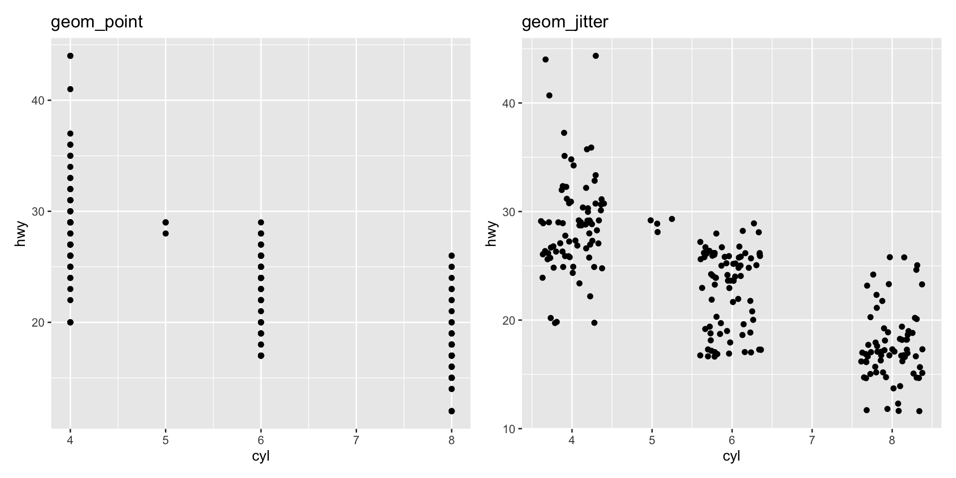
FAQ: Overplotting
Jitter: add a bit of random noise so points don’t step on each other
library(ggplot2); library(patchwork)
p <- ggplot(mpg, aes(cyl, hwy))
p1 <- p + geom_point() + ggtitle("geom_point")
p2 <- p + geom_jitter() + ggtitle("geom_jitter")
p1 + p2
![]()
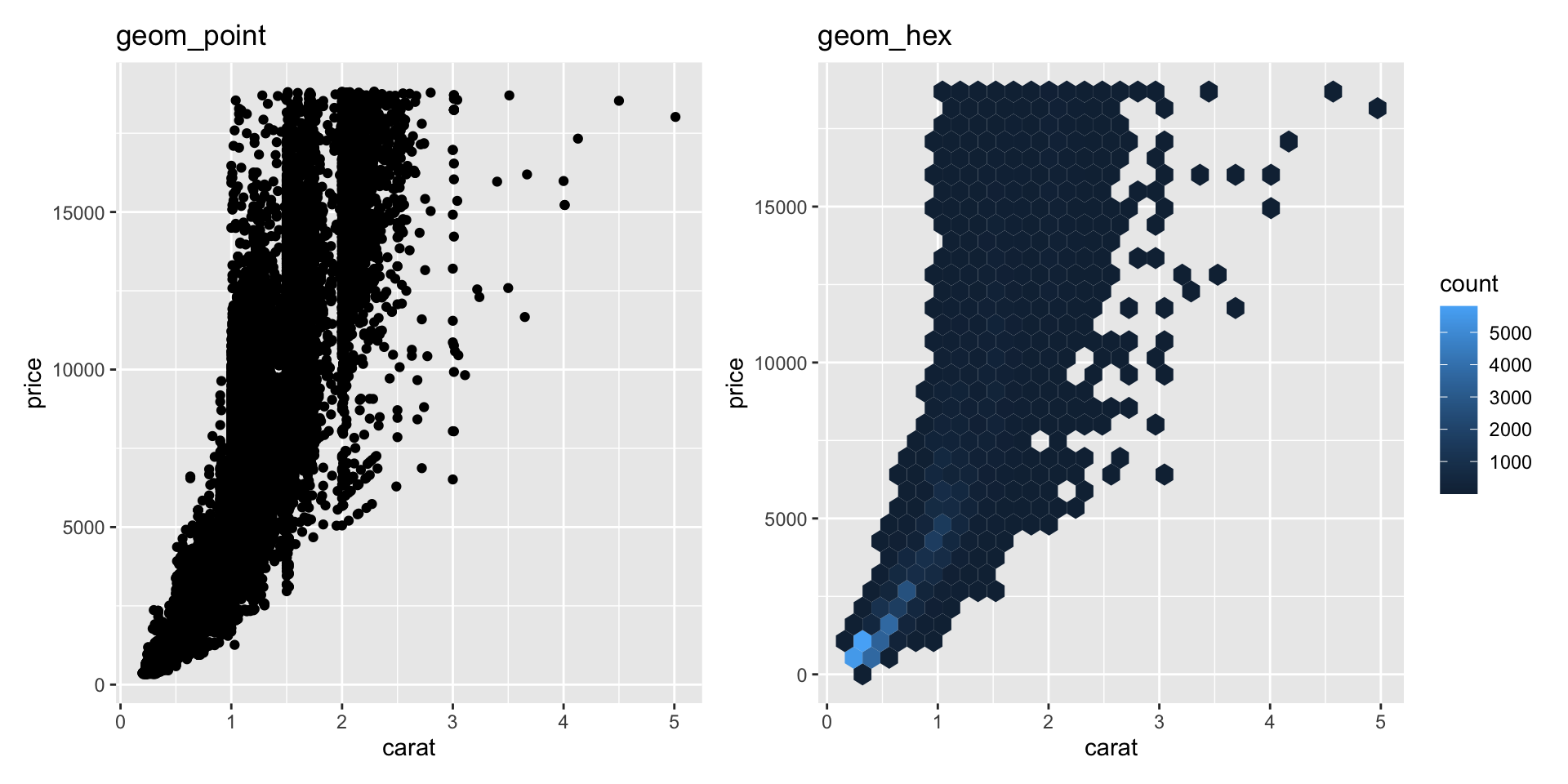
FAQ: Hexagonal Binning
Little “heatmaps” of counts. Hexagons to avoid weird rounding artifacts
library(ggplot2); library(patchwork)
p <- ggplot(diamonds, aes(carat, price))
p1 <- p + geom_point() + ggtitle("geom_point")
p2 <- p + geom_hex() + ggtitle("geom_hex")
p1 + p2
![]()
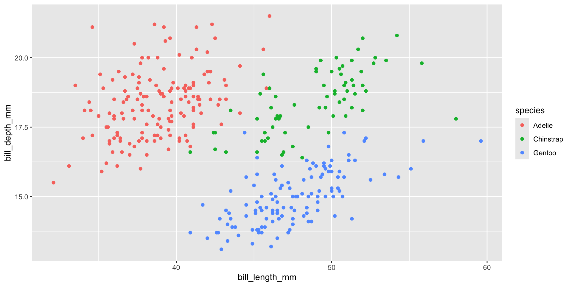
FAQ: Inside vs. Outside aes()
aes maps data to values. Outside of aes, set constant value
library(ggplot2); library(palmerpenguins)
ggplot(penguins,
       aes(x=bill_length_mm, y=bill_depth_mm, color=species))+ geom_point()
![]()
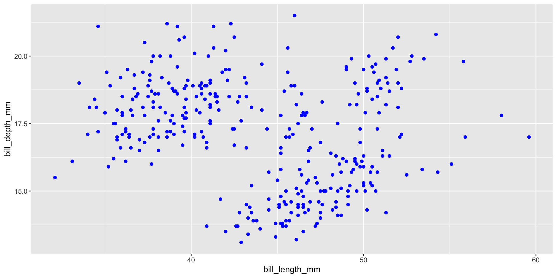
FAQ: Inside vs. Outside aes()
aes maps data to values. Outside of aes, set constant value
library(ggplot2); library(palmerpenguins)
ggplot(penguins,
       aes(x=bill_length_mm, y=bill_depth_mm))+ geom_point(color="blue")
![]()
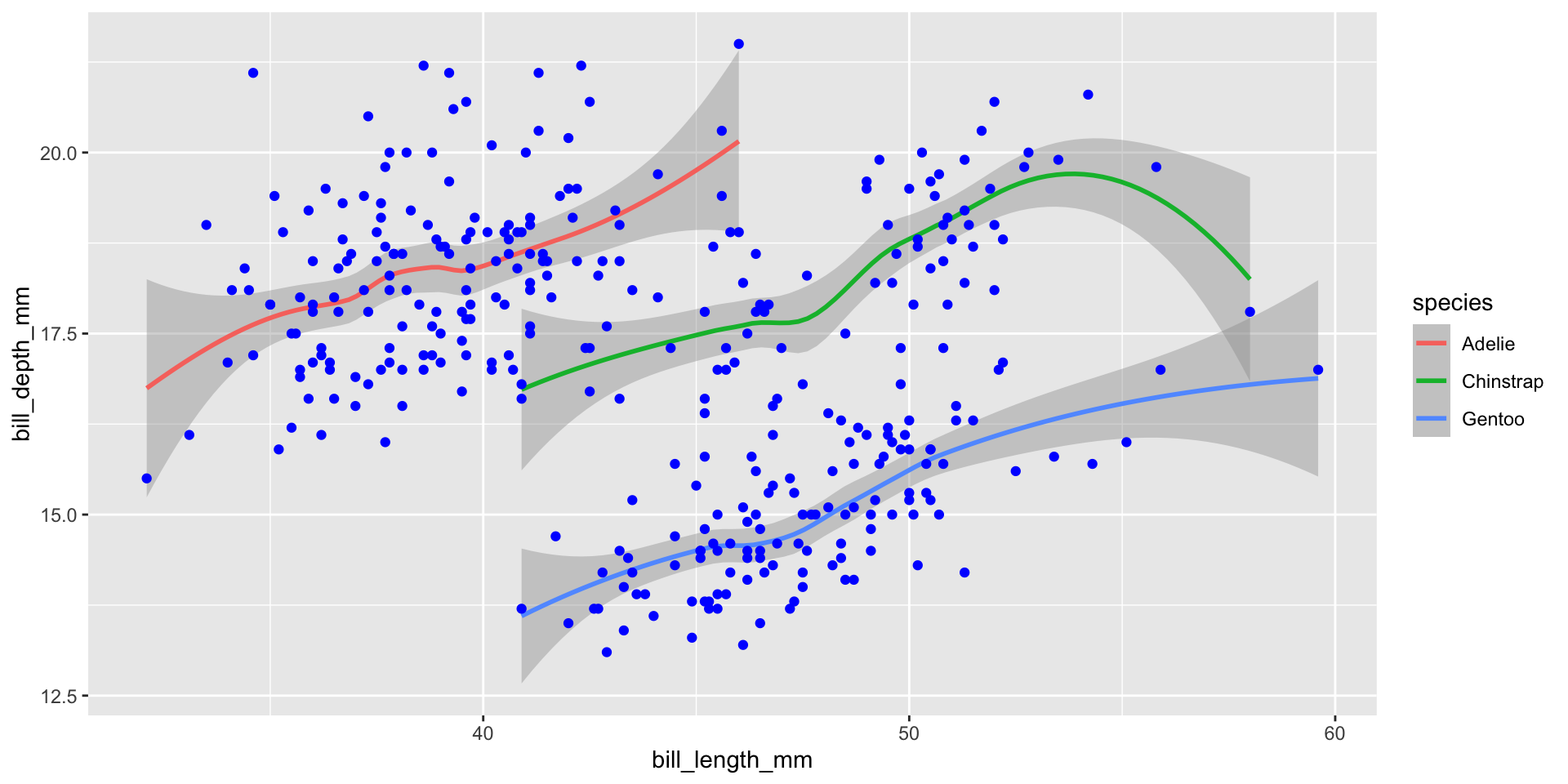
FAQ: Global vs geom_ specific aes()
- Elements set in
ggplot() apply to entire plot
- Elements set in specific
geom apply there only
library(ggplot2); library(palmerpenguins)
ggplot(penguins,
       aes(x=bill_length_mm, y=bill_depth_mm, color=species))+
    geom_smooth() +
    geom_point(color="blue")
![]()
FAQ: How to choose plot types
Two “modes”
- Exploratory data analysis. Quick, rapid iteration, for your eyes only
- Let the data tell you a story
- Low pre-processing: scatter plots, lines, histograms
- “Publication quality”. Polished,
- You tell the reader a story
- More processing, more modeling: trends, line segments, ribbons
FAQ: Color Palettes
Three types of color palettes:
- Sequential: ordered from 0 to “high”
- Example: rain forecast in different areas
- Diverging: ordered from -X to +X with meaningful 0 in the middle
- Example: political leaning
- Qualitative: no ordering
When mapping quantitative variables to palettes (sequential/diverging), two approaches:
- Binned: \([0, 1)\) light green, \([1, 3)\) medium green; \([3, 5]\) dark green
- Continuous
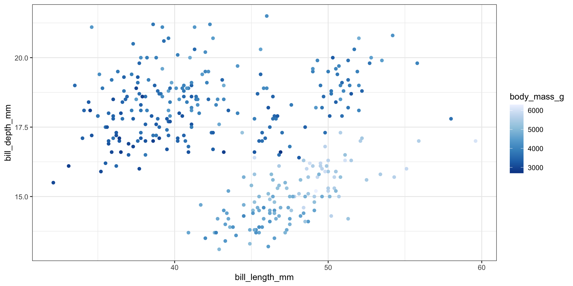
FAQ: Color Palettes
library(ggplot2); library(palmerpenguins)
ggplot(penguins, aes(x=bill_length_mm, y=bill_depth_mm, color=body_mass_g)) +
    geom_point() + theme_bw() +
    scale_color_distiller(type="seq") # Continuous
![]()
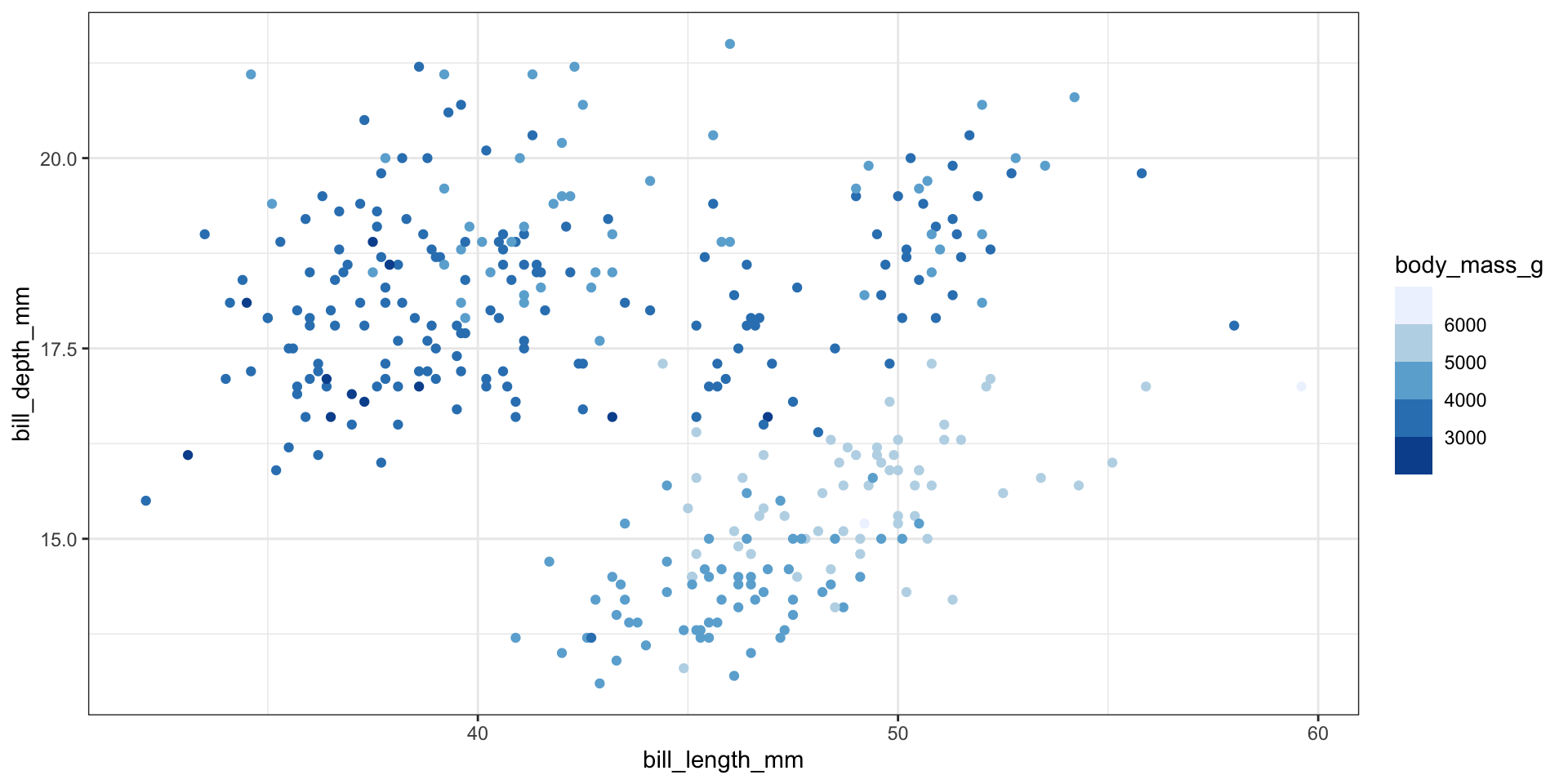
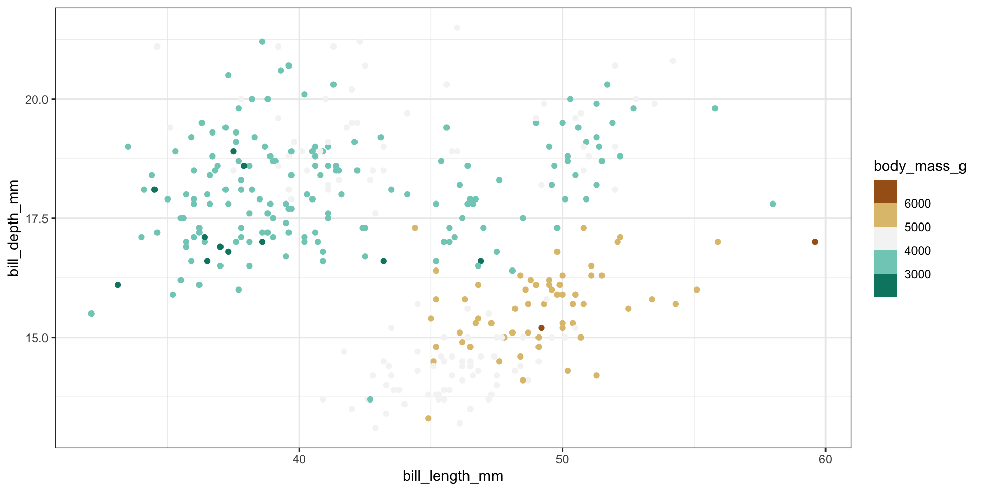
FAQ: Color Palettes
library(ggplot2); library(palmerpenguins)
ggplot(penguins, aes(x=bill_length_mm, y=bill_depth_mm, color=body_mass_g)) +
    geom_point() + theme_bw() +
    scale_color_fermenter(type="seq") # Binned
![]()
FAQ: Color Palettes
library(ggplot2); library(palmerpenguins)
ggplot(penguins, aes(x=bill_length_mm, y=bill_depth_mm, color=body_mass_g)) +
    geom_point() + theme_bw() +
    scale_color_fermenter(type="seq") # Binned + Sequential
![]()
FAQ: Color Palettes
library(ggplot2); library(palmerpenguins)
ggplot(penguins, aes(x=bill_length_mm, y=bill_depth_mm, color=body_mass_g)) +
    geom_point() + theme_bw() +
    scale_color_fermenter(type="qual") # Binned + Qualitative
![]()
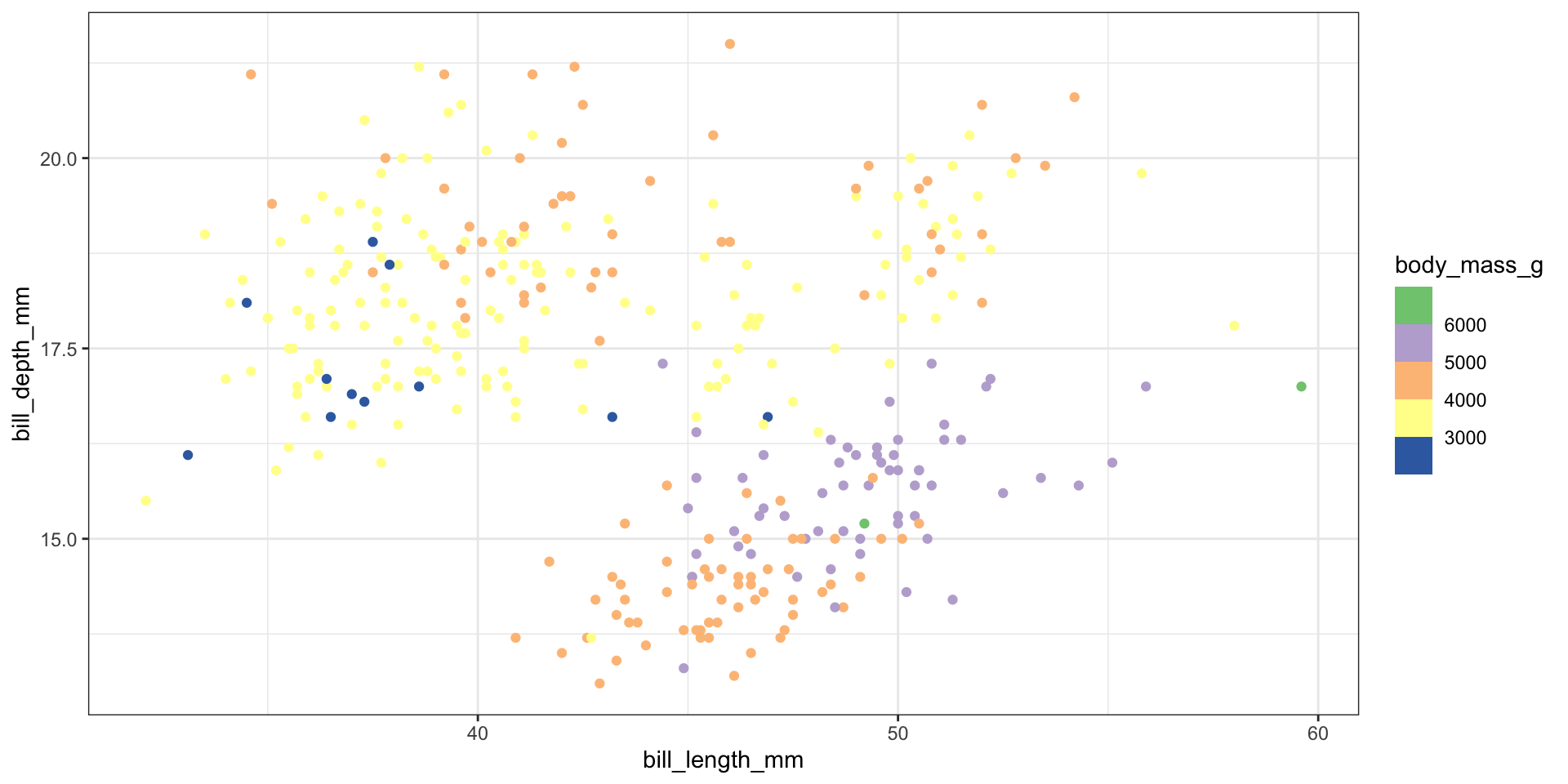
FAQ: Color Palettes
library(ggplot2); library(palmerpenguins)
ggplot(penguins, aes(x=bill_length_mm, y=bill_depth_mm, color=body_mass_g)) +
    geom_point() + theme_bw() +
    scale_color_fermenter(type="div") # Binned + Diverging
![]()
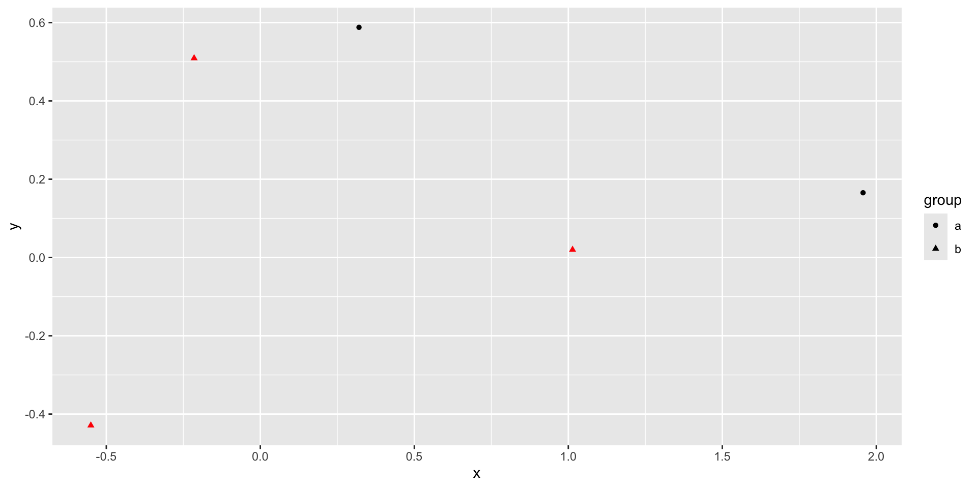
FAQ: How to “hard-code” colors
library(dplyr)
data <- data.frame(x = rnorm(5),
                   y = rnorm(5),
                   group = c("a", "a", "b", "b", "b"))

data |>
    group_by(group) |>
    mutate(n_count = n()) |>
    ungroup() |>
    mutate(color = ifelse(n_count == max(n_count), "red", "black")) |>
    ggplot(aes(x=x, y=y, shape=group, color=color)) +
    geom_point() +
    scale_color_identity()
![]()
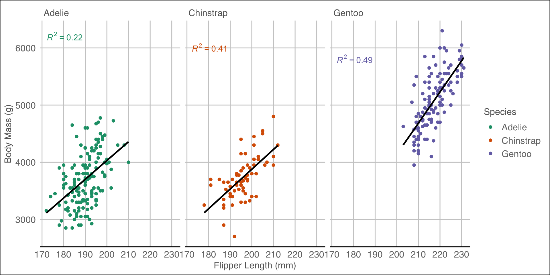
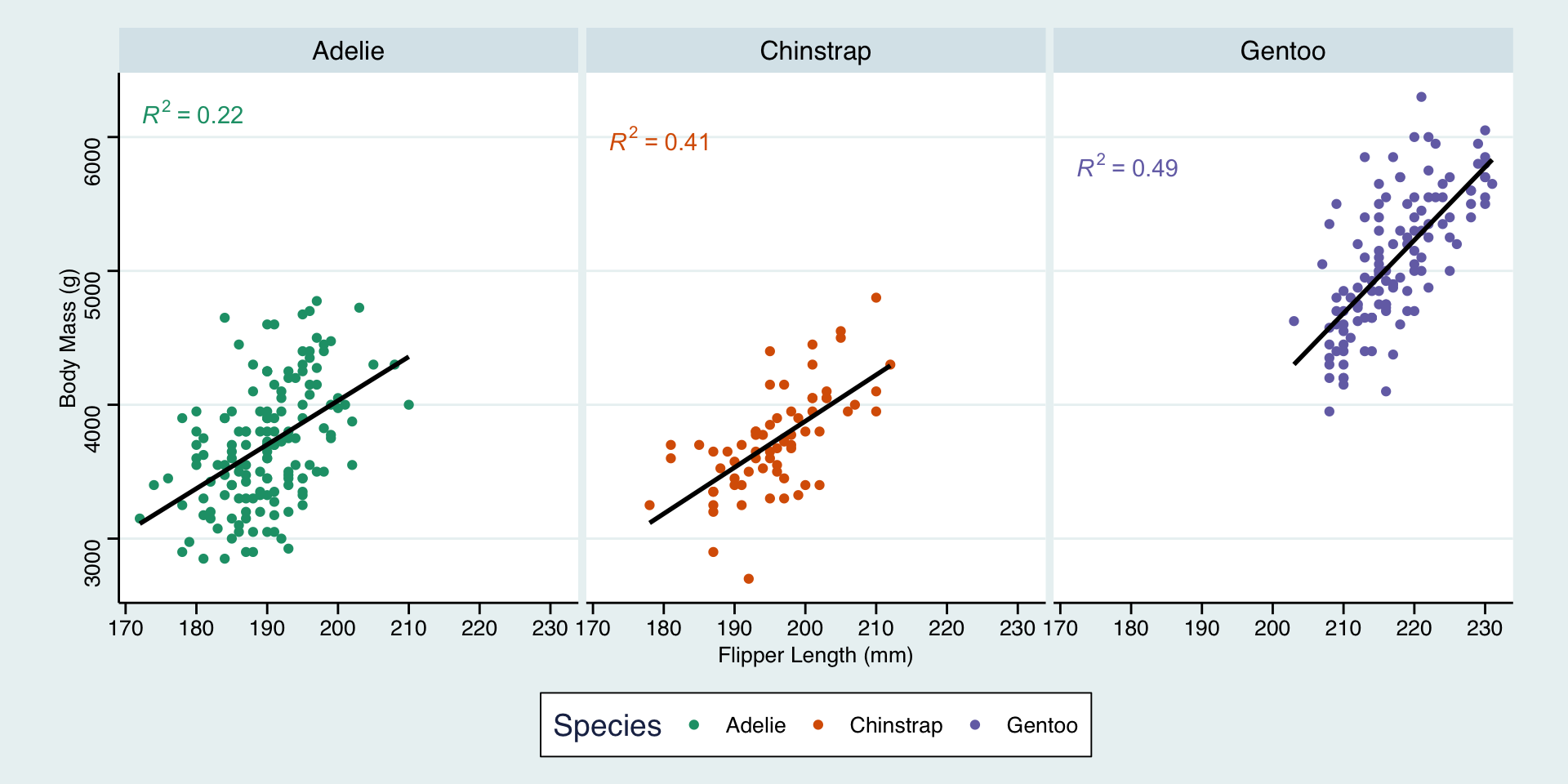
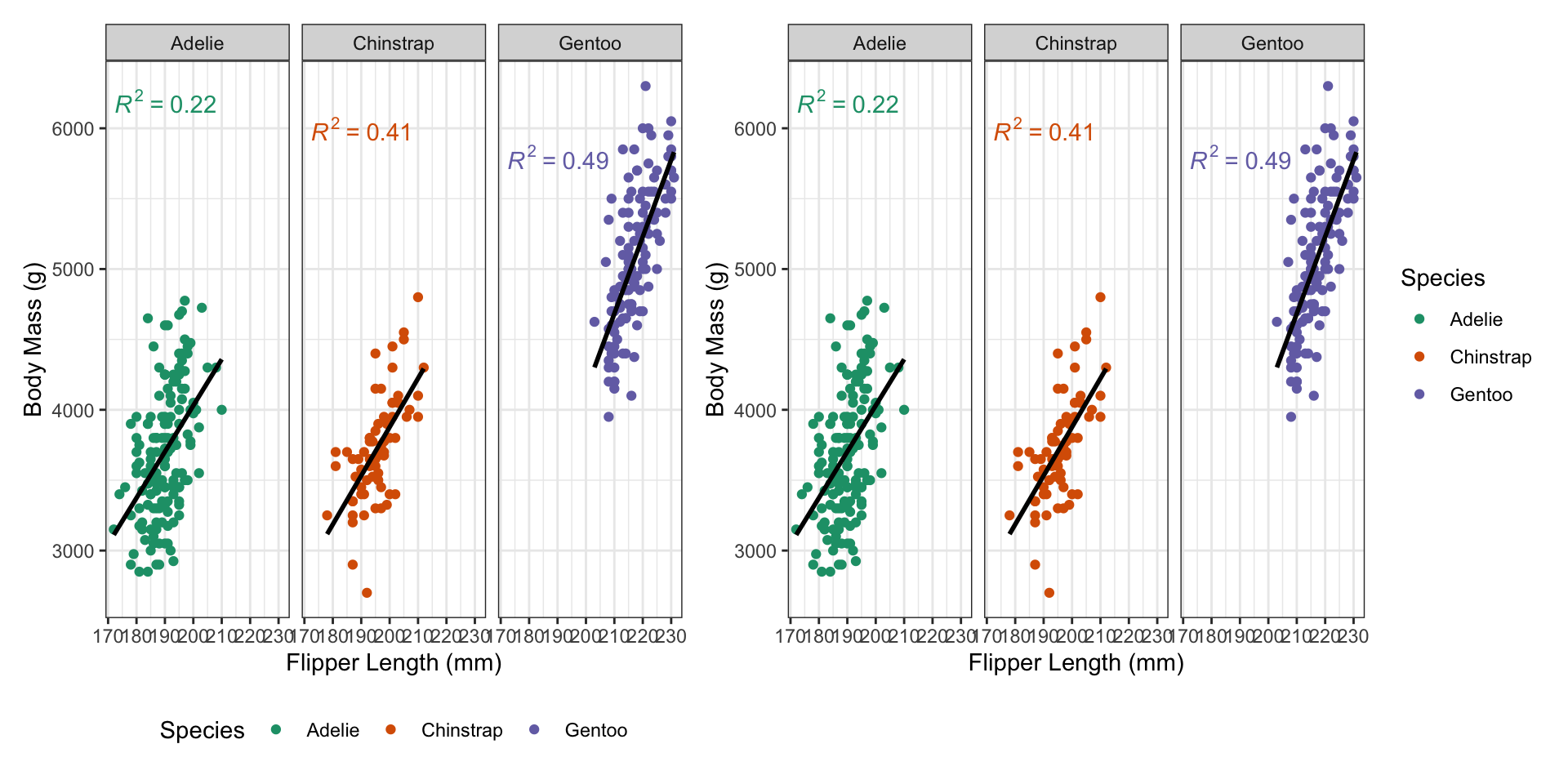
FAQ: How to Customize Themes
Built-in themes + ggthemes package:
library(ggplot2); library(ggthemes);
library(palmerpenguins); library(ggpmisc)
p <- ggplot(penguins,
       aes(x=flipper_length_mm,
           y=body_mass_g,
           color=species)) +
    geom_point() +
    stat_poly_line(se=FALSE,
                   color="black") +
    stat_poly_eq() +
    xlab("Flipper Length (mm)") +
    ylab("Body Mass (g)") +
    scale_color_brewer(type="qual",
                       palette=2,
                       name="Species") +
    facet_wrap(~species)
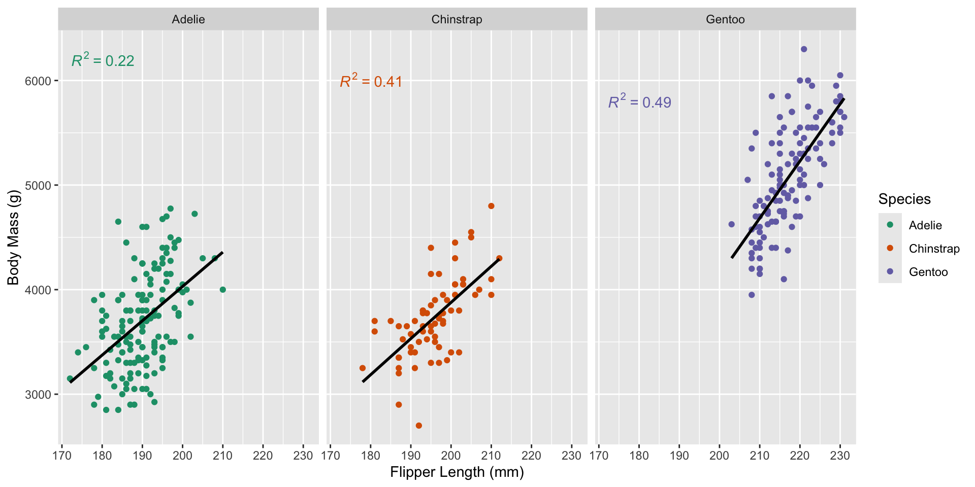
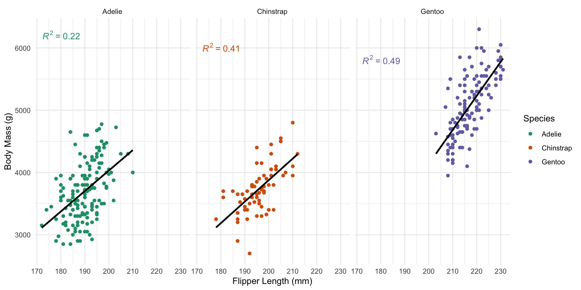
FAQ: Themes
Default theme (ggplot2::theme_grey()):
![]()
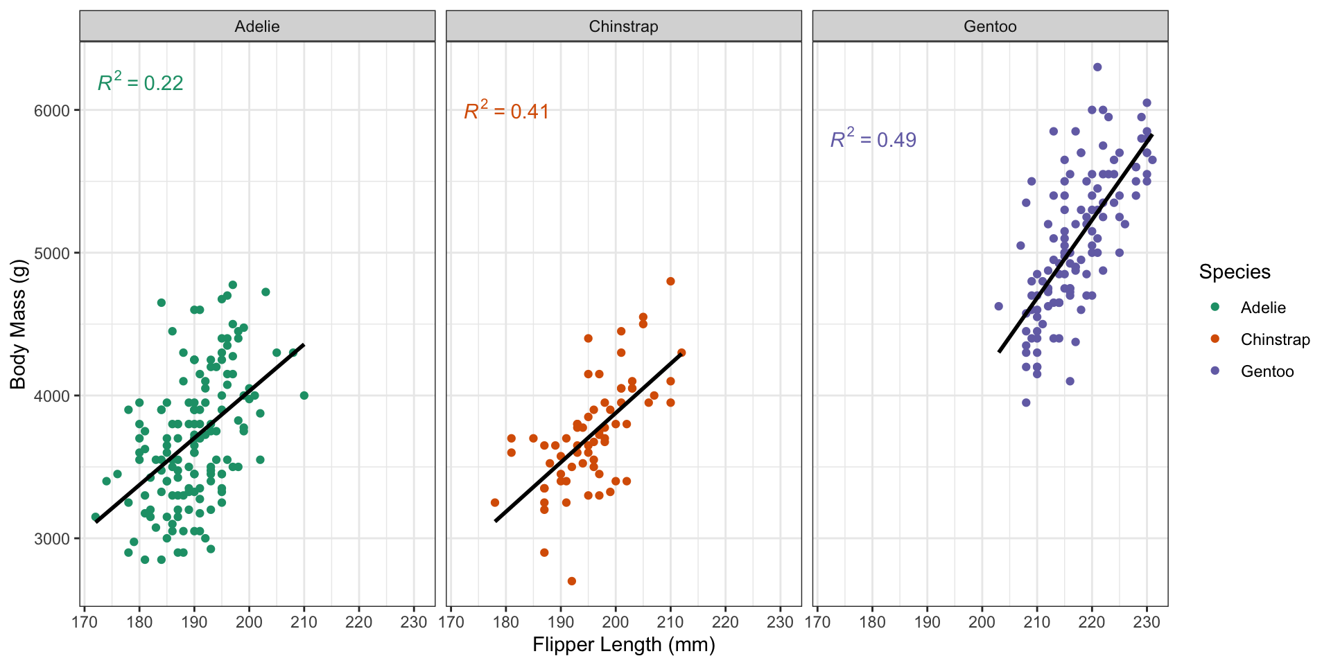
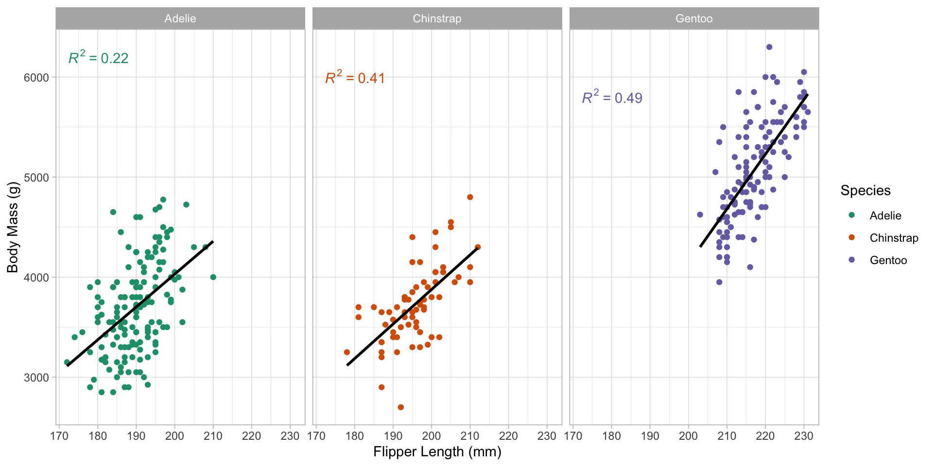
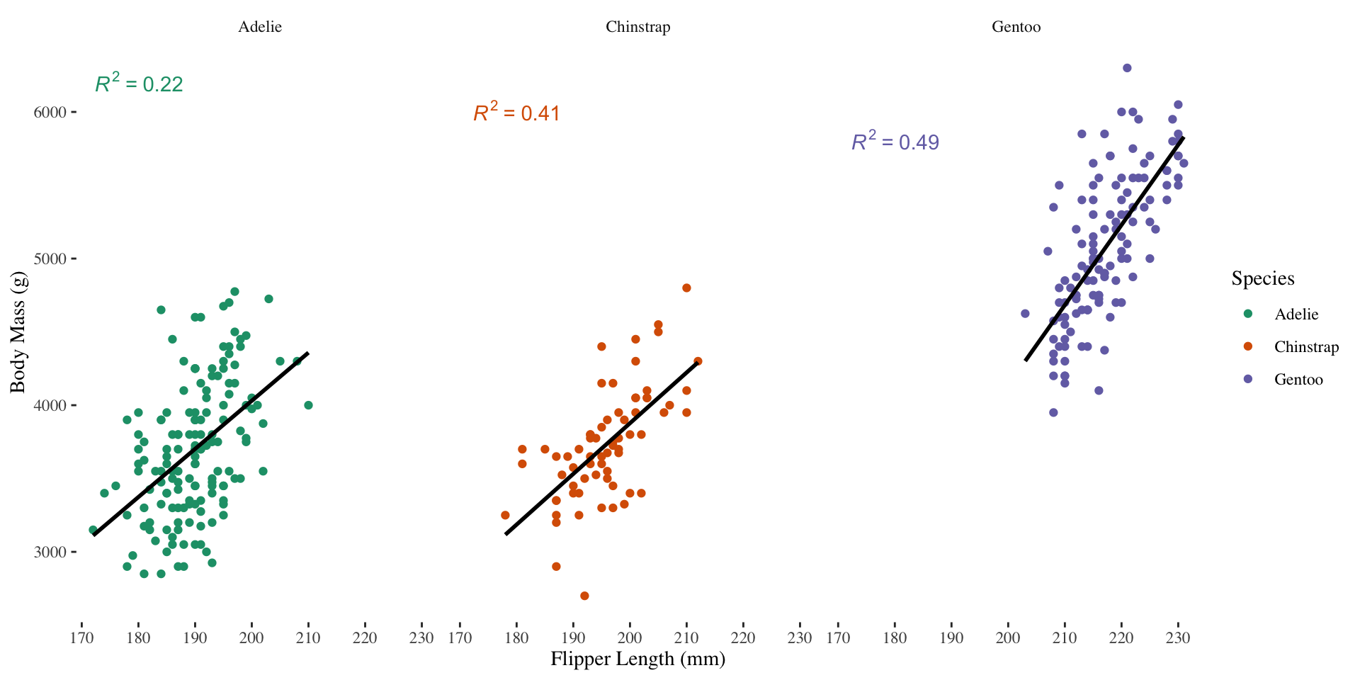
FAQ: Themes
Black and White theme (ggplot2::theme_bw()):
![]()
FAQ: Themes
Minimal theme (ggplot2::theme_minimal()):
![]()
FAQ: Themes
Light theme (ggplot2::theme_light()):
![]()
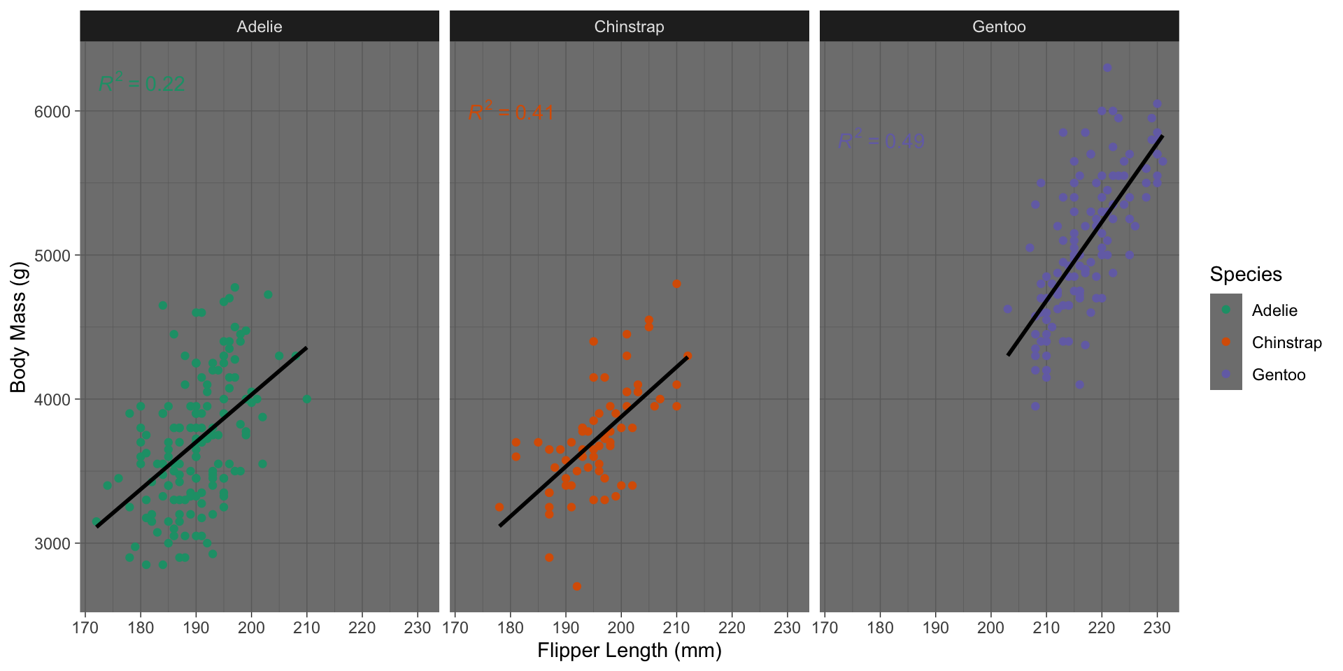
FAQ: Themes
Dark theme (ggplot2::theme_dark()):
![]()
FAQ: Themes
Excel theme (ggthemes::theme_excel()):
![]()
FAQ: Themes
Google Docs theme (ggthemes::theme_gdocs()):
![]()
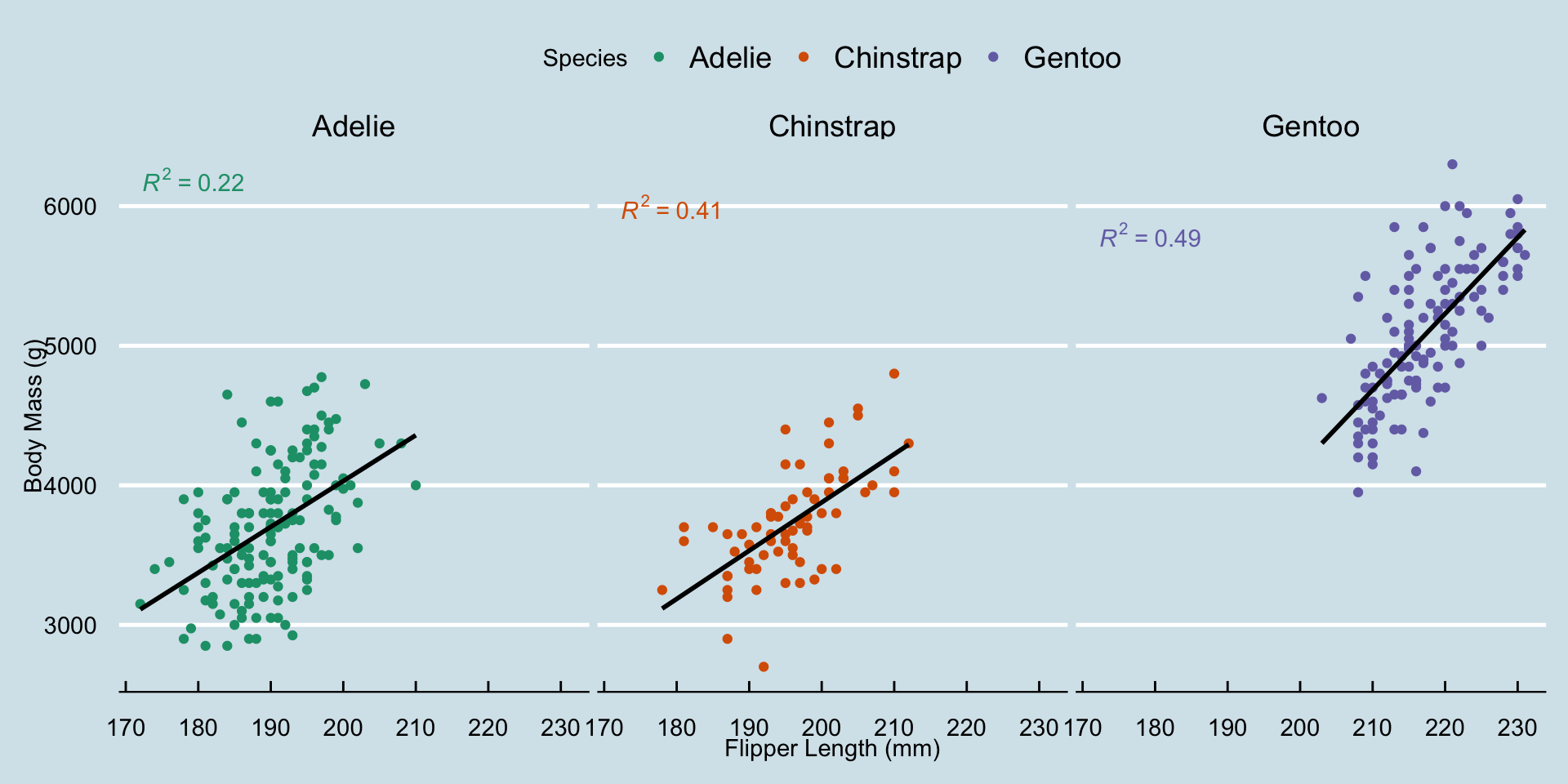
FAQ: Themes
The Economist theme (ggthemes::theme_economist()):
![]()
FAQ: Themes
The Economist theme (ggthemes::theme_economist()):
![]()
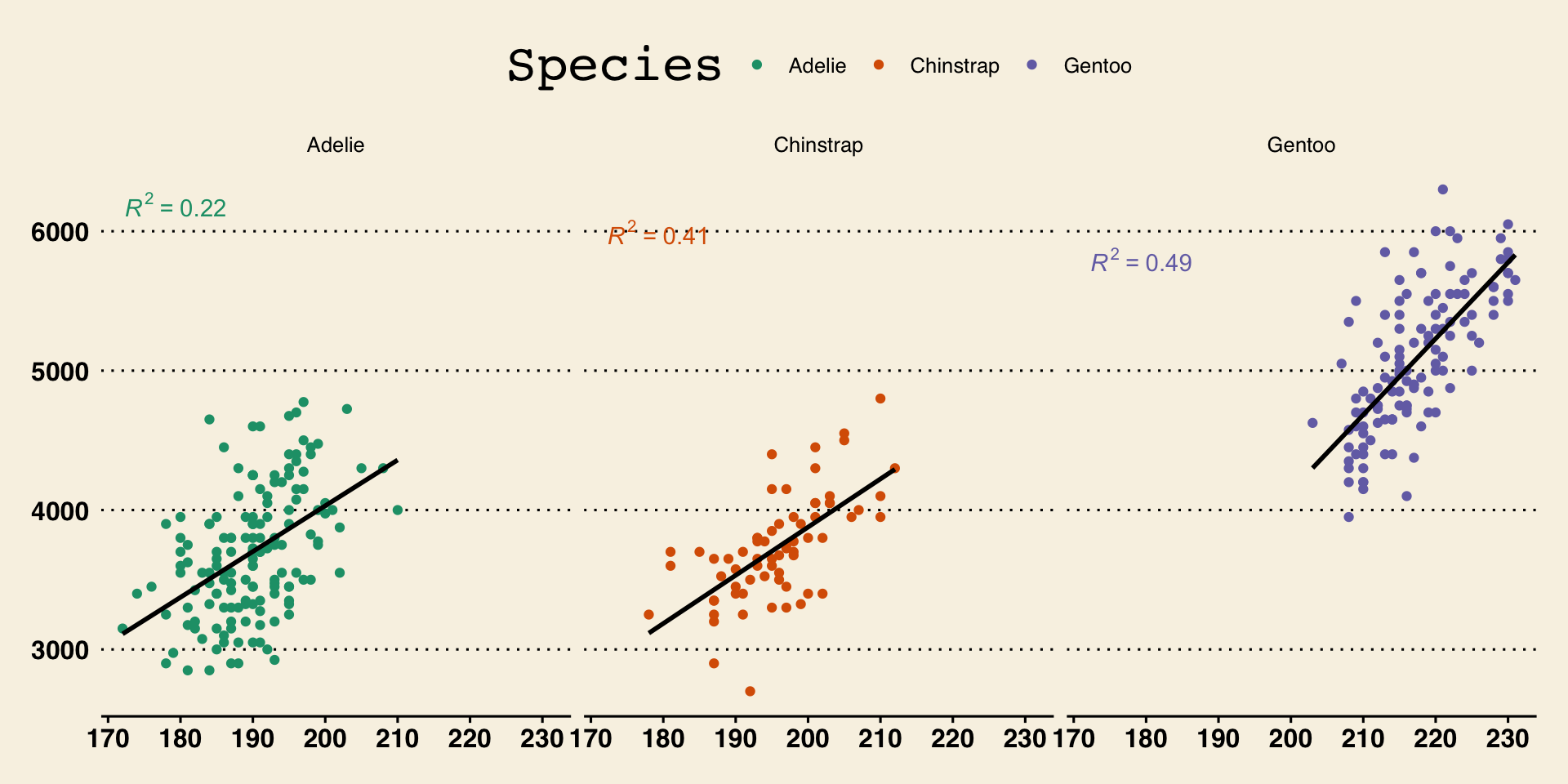
FAQ: Themes
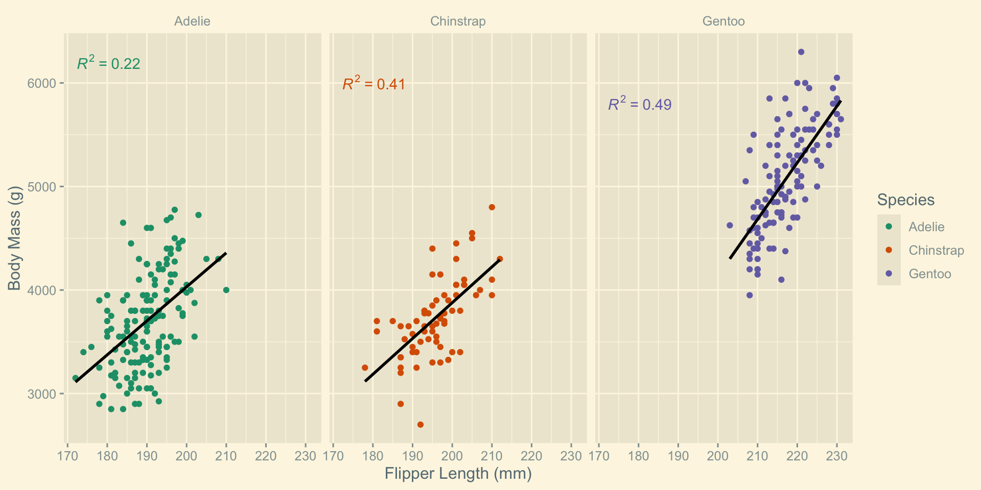
Solarized theme (ggthemes::theme_solarized()):
![]()
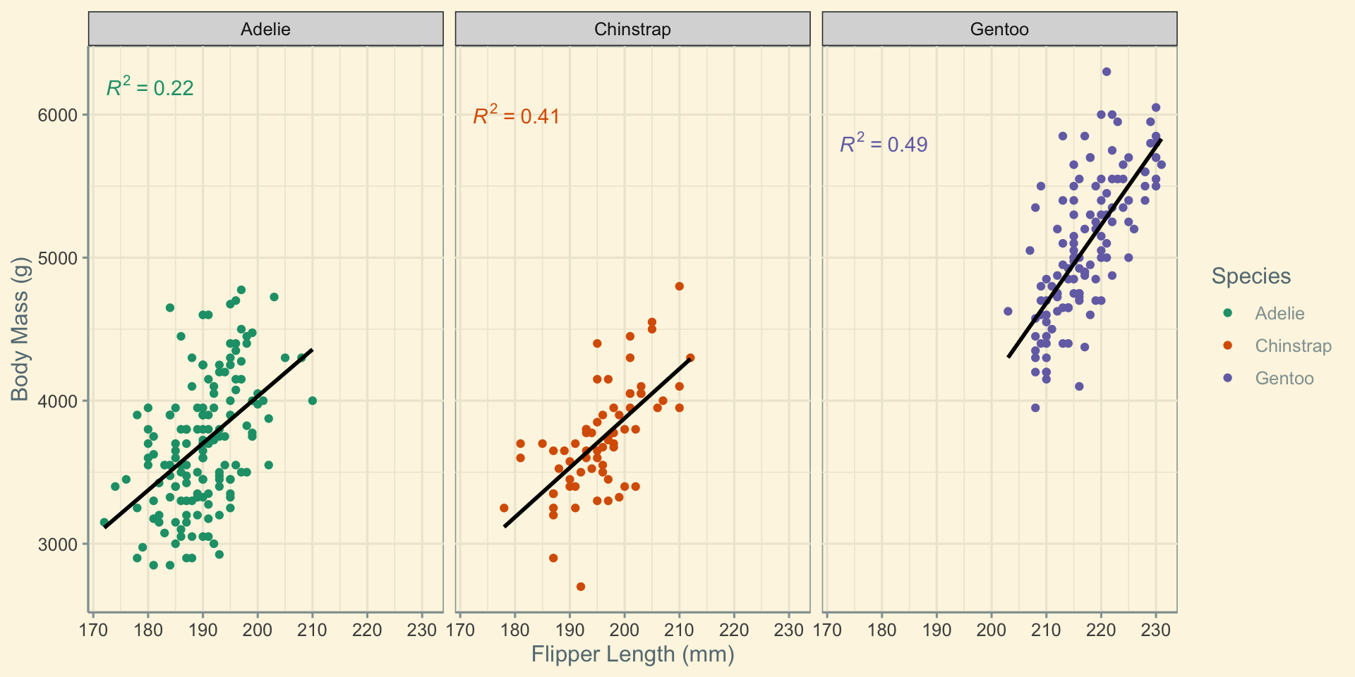
FAQ: Themes
Solarized2 theme (ggthemes::theme_solarized_2()):
![]()
FAQ: Themes
Stata theme (ggthemes::theme_stata()):
![]()
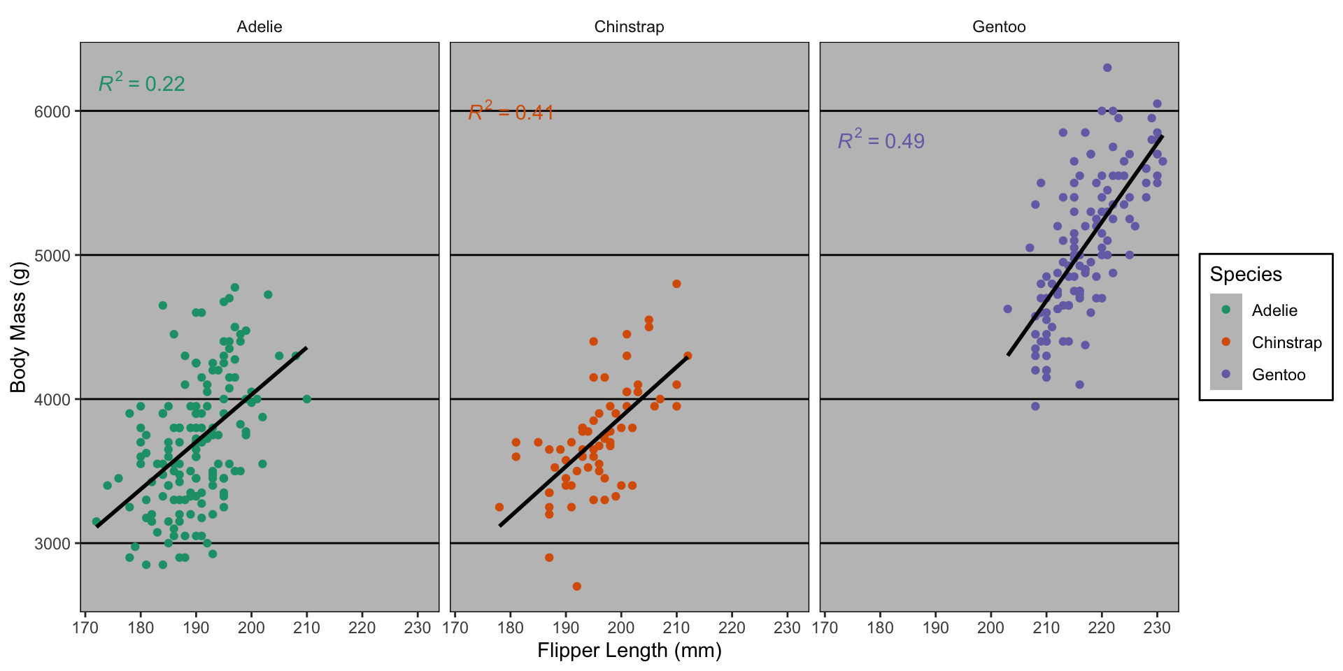
FAQ: Themes
Tufte theme (ggthemes::theme_tufte()):
![]()
FAQ: Themes
Wall Street Journal theme (ggthemes::theme_wsj()):
![]()
FAQ: Themes
Many more online:
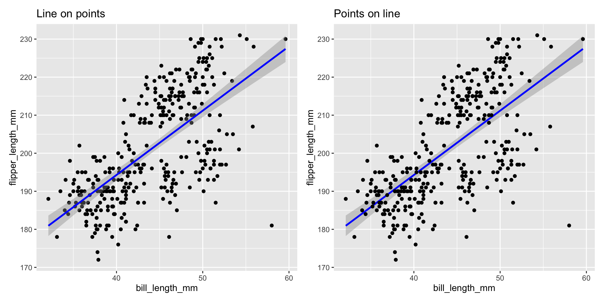
FAQ: Order of Layers
Order of layers technically matters, but the effect is small
p1 <- ggplot(penguins, aes(x=bill_length_mm, y=flipper_length_mm)) +
        geom_point(color="black") +
        geom_smooth(color="blue", method="lm") + ggtitle("Line on points")
p2 <- ggplot(penguins, aes(x=bill_length_mm, y=flipper_length_mm)) +
        geom_smooth(color="blue", method="lm") +
        geom_point(color="black") + ggtitle("Points on line")
p1 + p2
![]()
FAQ: Order of layers
Order matters more with theme. Adding a theme_*() will override any theme() customization you did:
p1 <- p + theme_bw() + theme(legend.position="bottom")
p2 <- p + theme(legend.position="bottom") + theme_bw()
p1 + p2
![]()
FAQ: stat_poly_{line,eq} vs geom_smooth
By default geom_smooth fits a generalized additive model (GAM)
ggpmisc::stat_poly_{line,eq} fit linear models, so they can expose more machinery.
What is a GAM? Take 9890 with me (Spring, Tuesdays at 6) to find out!
FAQ: Titles and Captions
ggplot() +
    labs(title="Title", subtitle="Subtitle", caption="Caption",
         tag="Tag", alt="Alt-Text", alt_insight="Alt-Insight")
![]()
+ggtitle("text") is just shorthand for +labs(title="text")
FAQ: Relative Importance of Aesthetics
Perceptually:
- Location > Color > Size > Shape
Humans are better at:
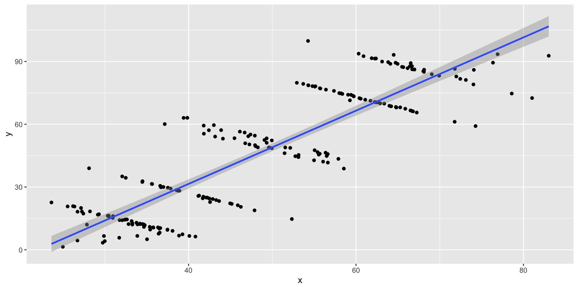
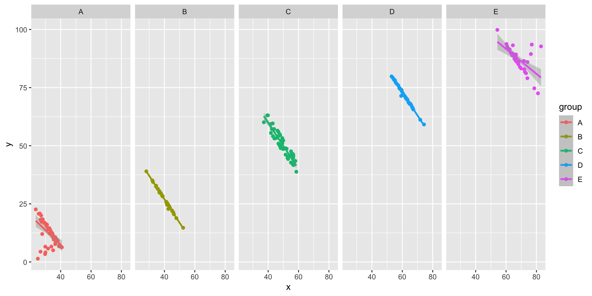
FAQ: When to Use Facets?
Facets are group_by for plots. Useful for
- Distinguishing intra- vs inter-group trends
- Avoiding overplotting
FAQ: Simpson’s Paradox
![]()
FAQ: Simpson’s Paradox
![]()
FAQ: Twin Axes Plots
How can I implement a dual (twin) axis plot in ggplot2?
Disfavored. But if you must …
sec.axis
Doesn’t allow arbitrary secondary axes; allows transformed axes (e.g., Celsius and Fahrenheit)
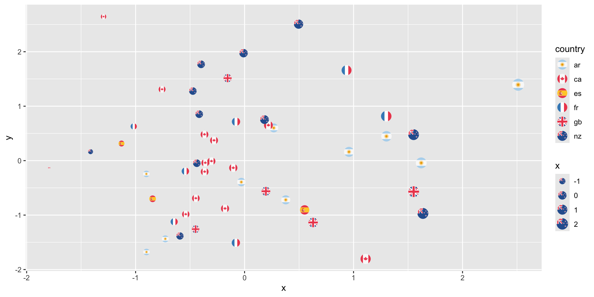
FAQ: Embedding images in ggplot
See the ggimage or ggflags package for images as “points”:
#devtools::install_github("jimjam-slam/ggflags");
library(ggflags)
d <- data.frame(x=rnorm(50), y=rnorm(50),
                country=sample(c("ar","fr", "nz", "gb", "es", "ca"), 50, TRUE),
                stringsAsFactors = FALSE)
ggplot(d, aes(x=x, y=y, country=country, size=x)) +
  geom_flag() +
  scale_country()
![]()
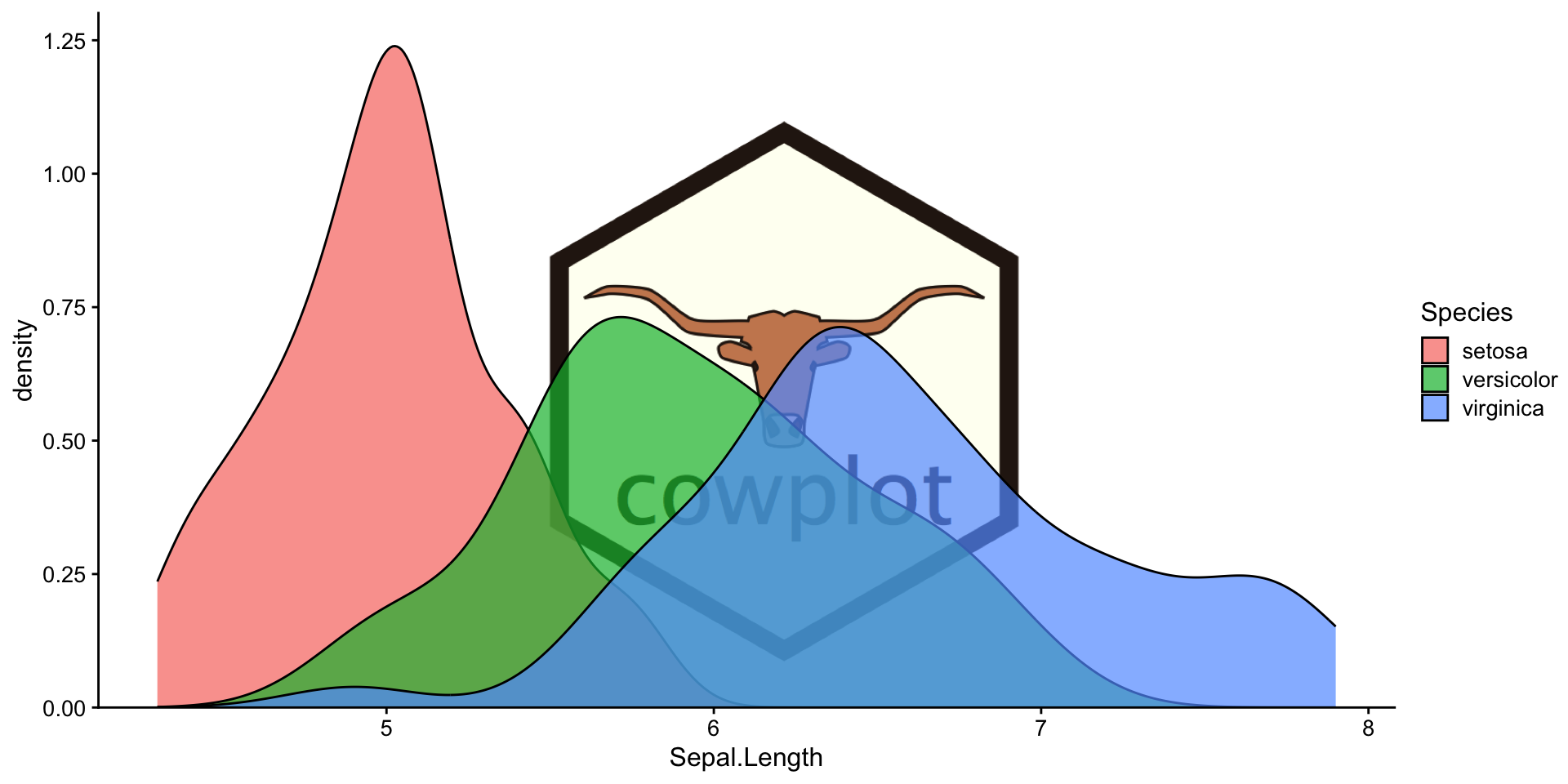
FAQ: Embedding Images
See cowplot::draw_image() for image background:
library(cowplot)
p <- ggplot(iris, aes(x = Sepal.Length, fill = Species)) +
  geom_density(alpha = 0.7) +
  scale_y_continuous(expand = expansion(mult = c(0, 0.05))) +
  theme_half_open(12)

logo_file <- system.file("extdata", "logo.png", package = "cowplot")
ggdraw() +
  draw_image(
    logo_file, scale = .7
  ) +
  draw_plot(p)
![]()