STA 9750 Mini-Project #02
A few students have reported issues with rate-limiting on the EIA SEP site. Re-running the code seems to resolve issues.
My download code is written to save the files locally, so only needs to succeed once.
One student reported NA conversion warnings in processing the NTD data. These were harmless, but I’ve modified the provided code to suppress these warnings.
In brief: update to NTD now uses dashes in a few places for missing data and NA warning came up when trying to conver these to numeric values
FAQ: ggplot2 vs Tableau
Tableau
$$$
IT department automatically integrates with data sources
Easy, if it does what you want
ggplot2
Free
Can use arbitrary data sources, with effort
Flexible / customizable
FAQ: ggplot2 vs matplotlib
ggplot2
Data visualizations
Enforces “good practice” via gg
matplotlib
Scientific visualizations
More flexible for good or for ill
Inspired by Matlab plotting
Closest Python analogue to ggplot2 is seaborn
FAQ: Why use + instead of |>
ggplot2 is older than |>
Per H. Wickham: if ggplot3 ever gets made, will use |>
Unlikely to change: too much code depends on it
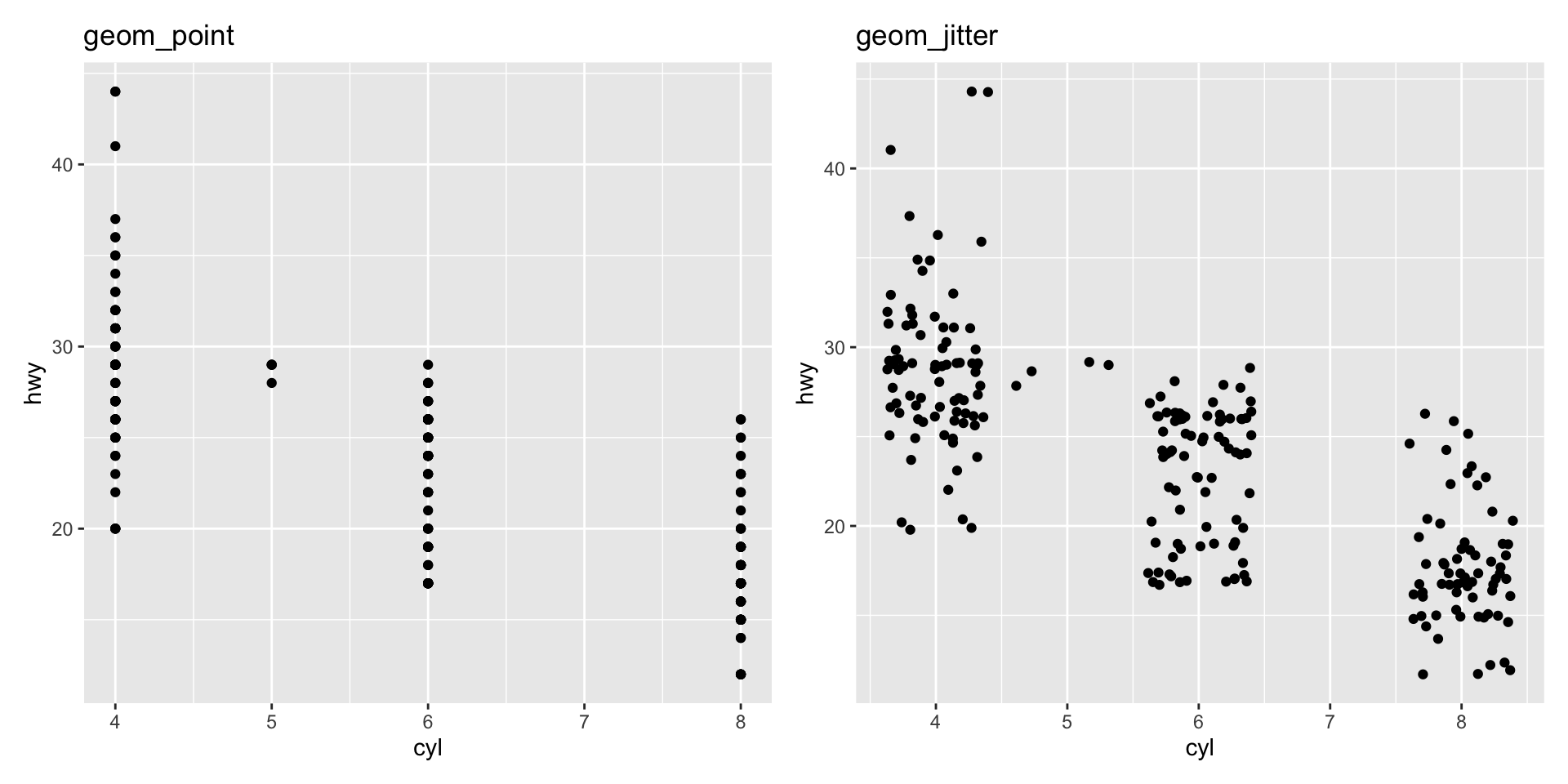
FAQ: Overplotting
Large data sets can lead to overplotting :
Points “on top of” each other
Can also occur with “designed” experiments / rounded data
Ways to address:
FAQ: Overplotting
Jitter: add a bit of random noise so points don’t step on each other
library (ggplot2); library (patchwork)<- ggplot (mpg, aes (cyl, hwy))<- p + geom_point () + ggtitle ("geom_point" )<- p + geom_jitter () + ggtitle ("geom_jitter" )+ p2
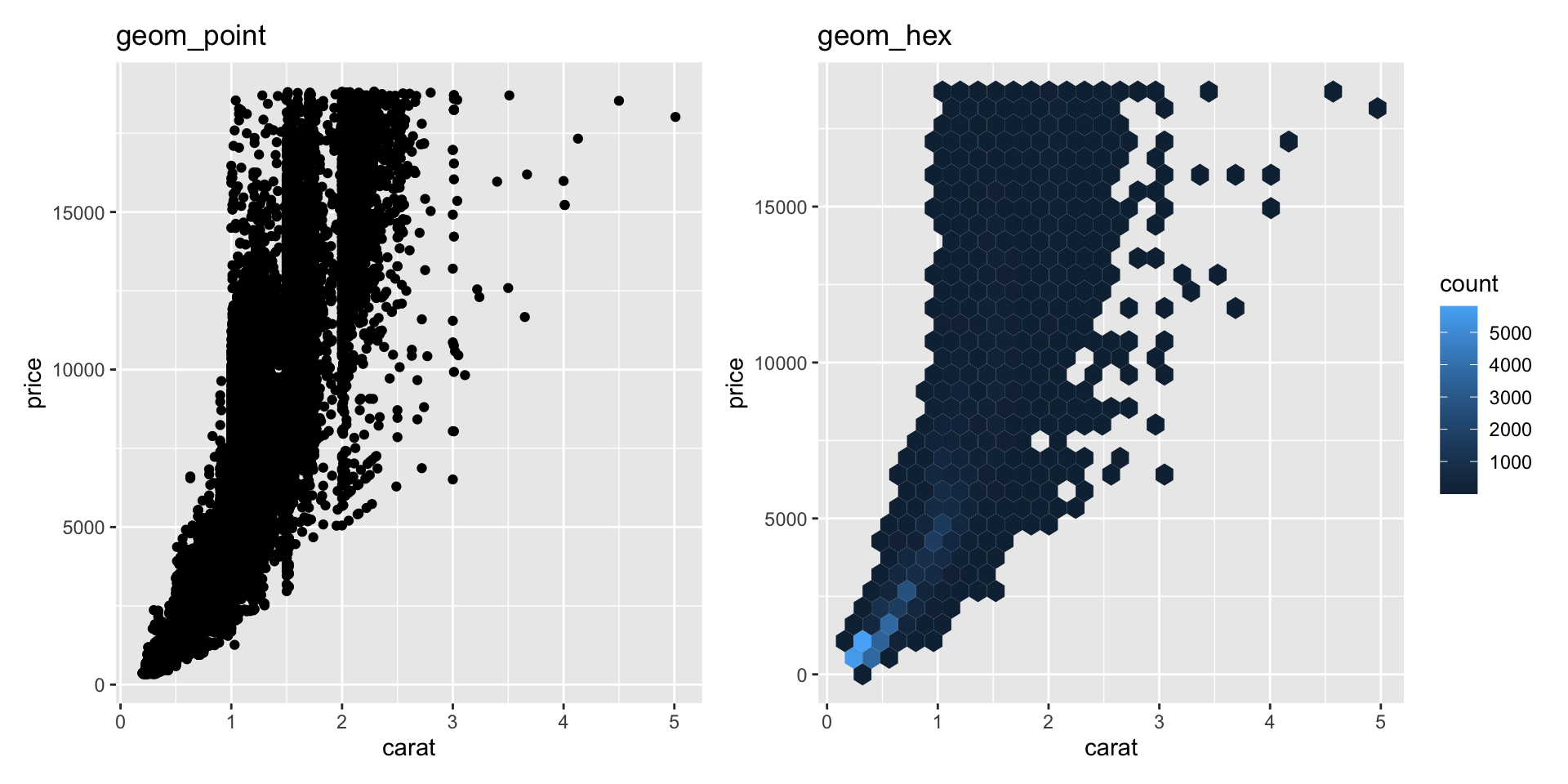
FAQ: Hexagonal Binning
Little “heatmaps” of counts. Hexagons to avoid weird rounding artifacts
library (ggplot2); library (patchwork)<- ggplot (diamonds, aes (carat, price))<- p + geom_point () + ggtitle ("geom_point" )<- p + geom_hex () + ggtitle ("geom_hex" )+ p2
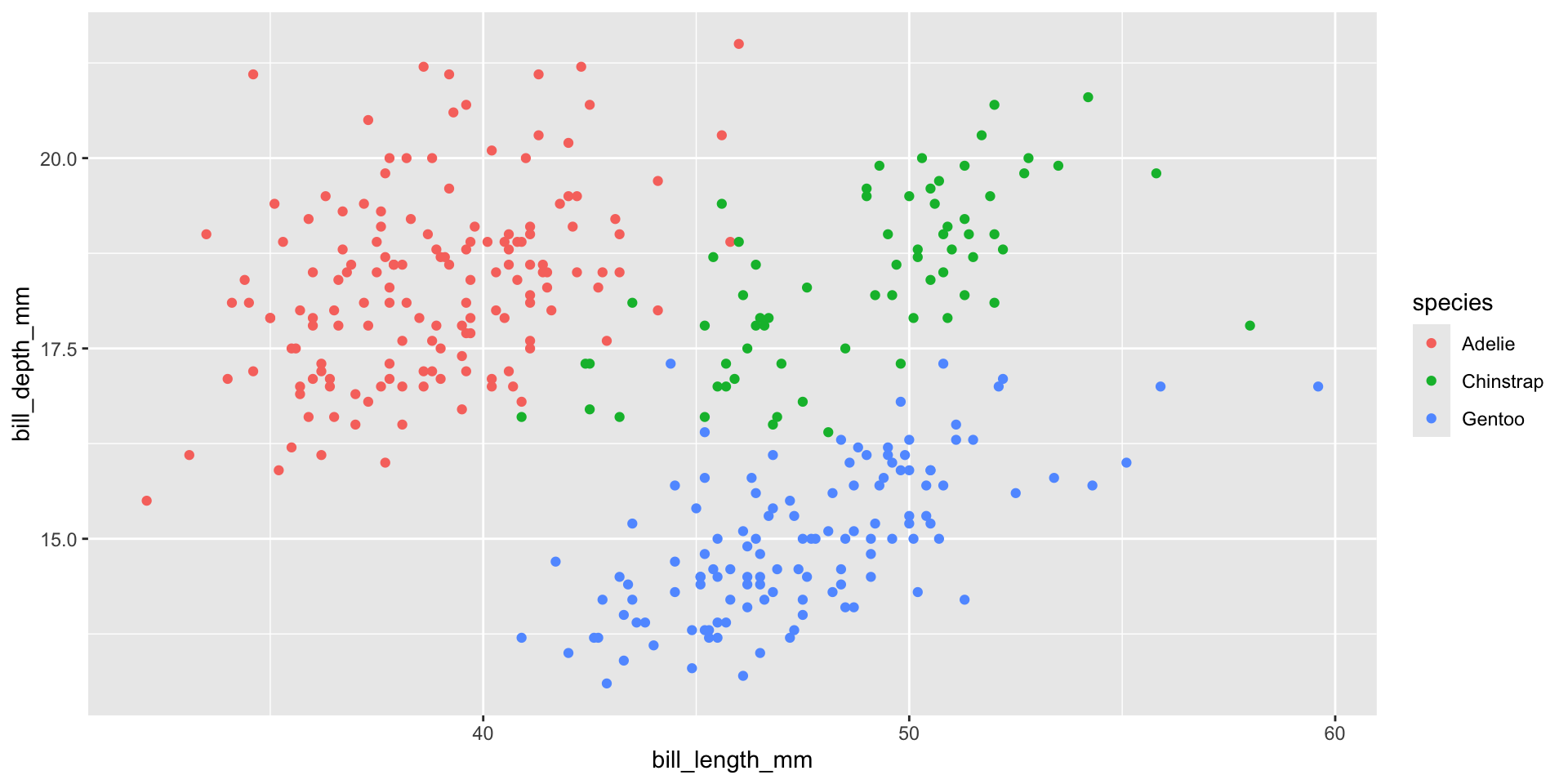
FAQ: Inside vs. Outside aes()
aes maps data to values . Outside of aes, set constant value
library (ggplot2); library (palmerpenguins)ggplot (penguins, aes (x= bill_length_mm, y= bill_depth_mm, color= species))+ geom_point ()
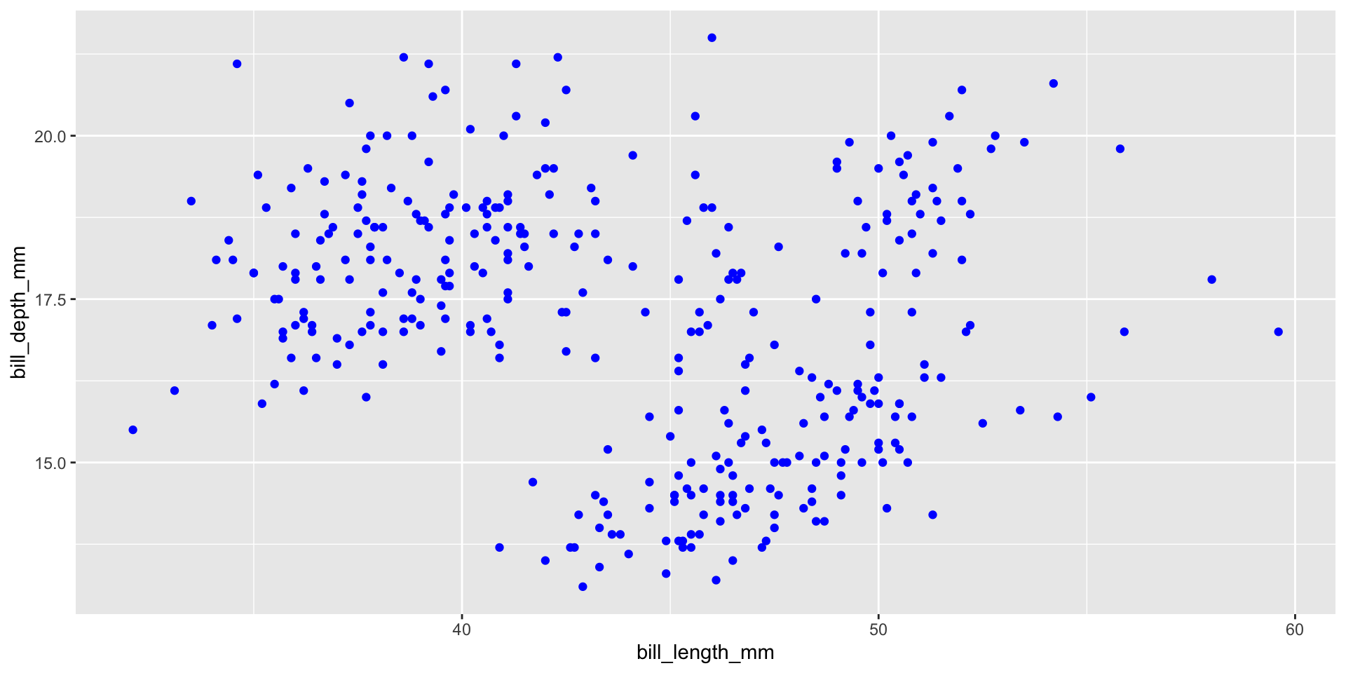
FAQ: Inside vs. Outside aes()
aes maps data to values . Outside of aes, set constant value
library (ggplot2); library (palmerpenguins)ggplot (penguins, aes (x= bill_length_mm, y= bill_depth_mm))+ geom_point (color= "blue" )
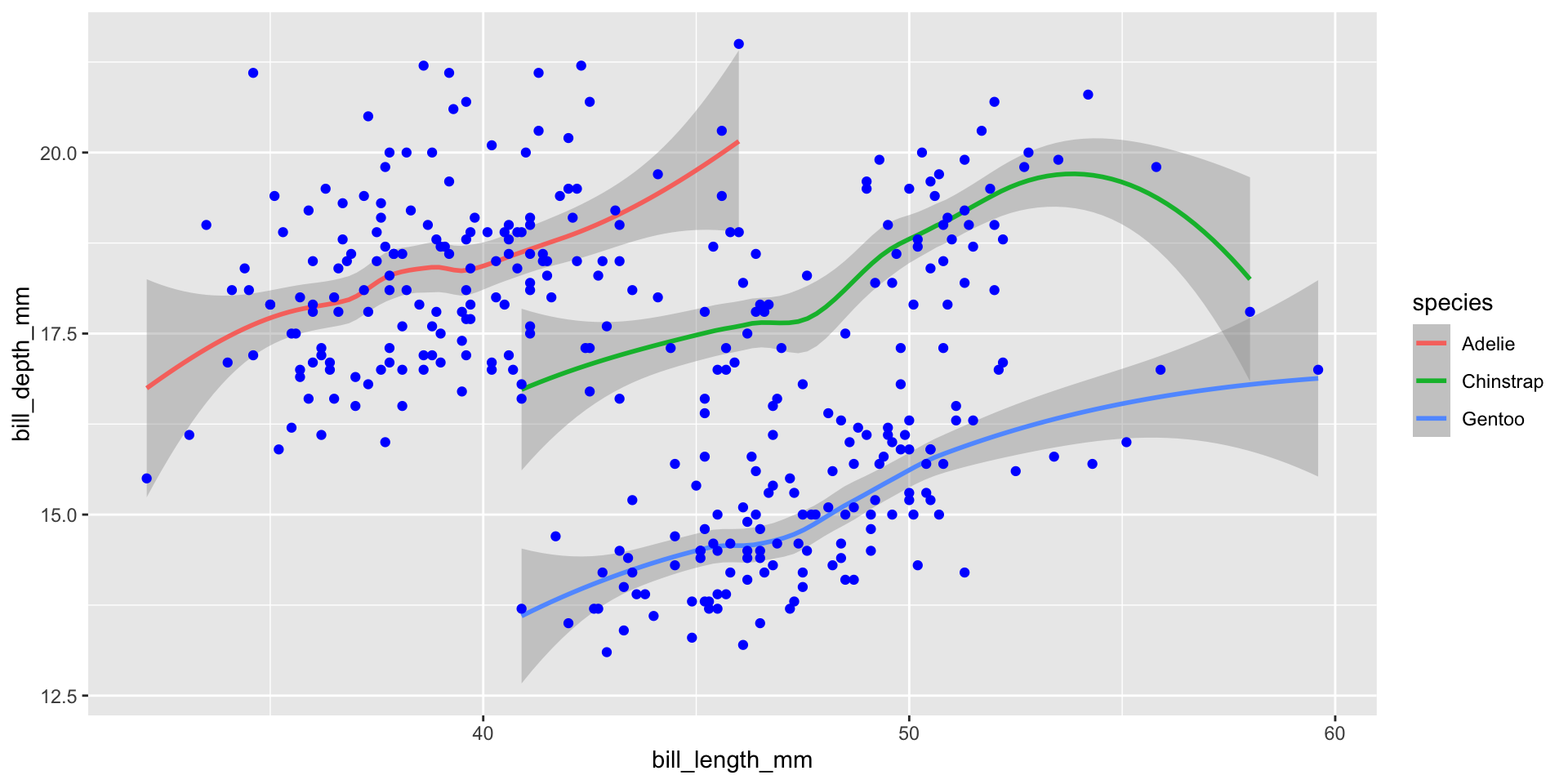
FAQ: Global vs geom_ specific aes()
Elements set in ggplot() apply to entire plot
Elements set in specific geom apply there only
library (ggplot2); library (palmerpenguins)ggplot (penguins, aes (x= bill_length_mm, y= bill_depth_mm, color= species))+ geom_smooth () + geom_point (color= "blue" )
FAQ: How to choose plot types
Two “modes”
Exploratory data analysis. Quick, rapid iteration, for your eyes only
Let the data tell you a story
Low pre-processing: scatter plots, lines, histograms
“Publication quality”. Polished,
You tell the reader a story
More processing, more modeling: trends, line segments, ribbons
FAQ: Color Palettes
Three types of color palettes:
Sequential: ordered from 0 to “high”
Example: rain forecast in different areas
Diverging: ordered from -X to +X with meaningful 0 in the middle
Example: political leaning
Qualitative: no ordering
When mapping quantitative variables to palettes (sequential/diverging), two approaches:
Binned: \([0, 1)\) light green, \([1, 3)\) medium green; \([3, 5]\) dark green
Continuous
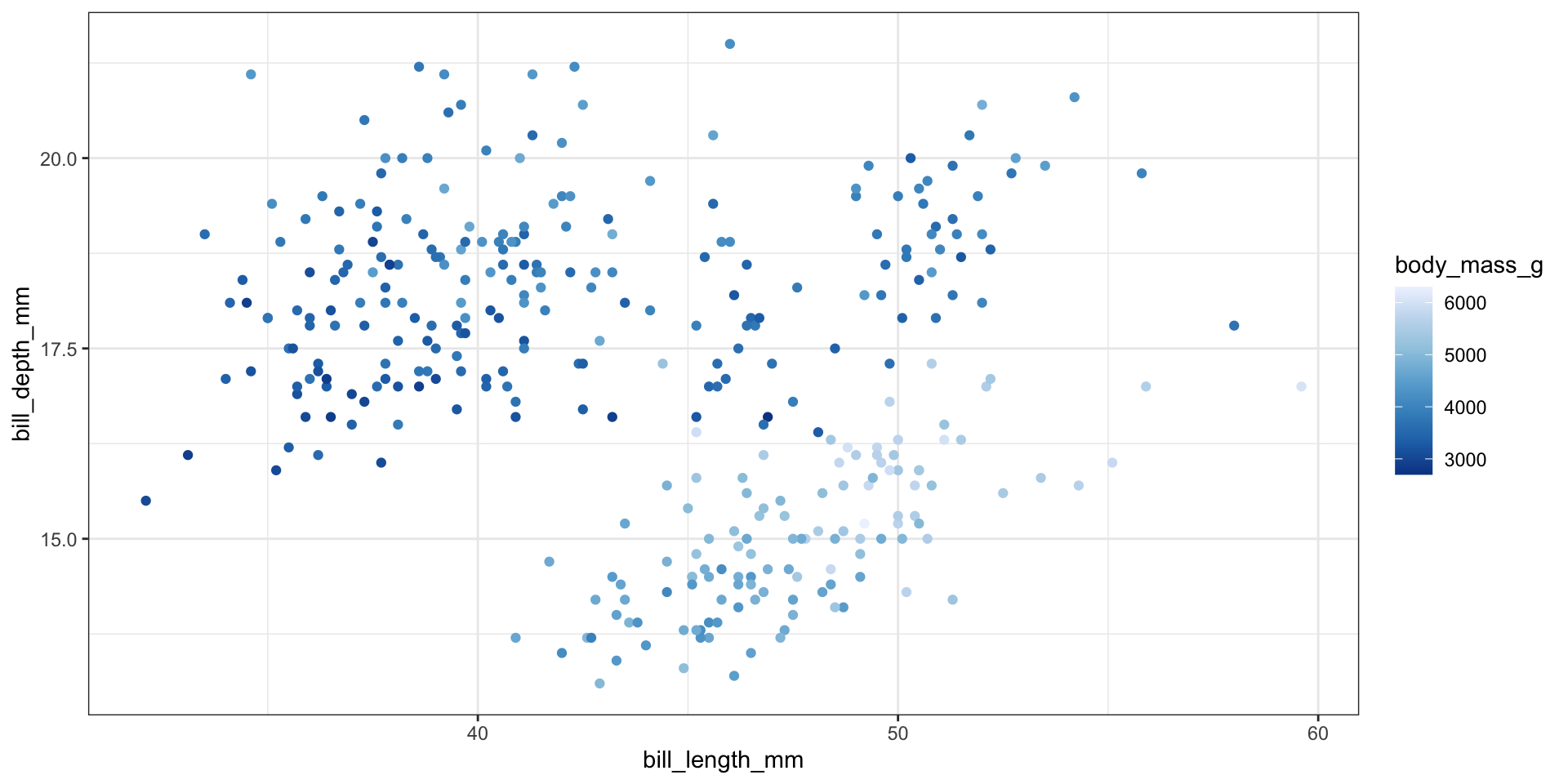
FAQ: Color Palettes
library (ggplot2); library (palmerpenguins)ggplot (penguins, aes (x= bill_length_mm, y= bill_depth_mm, color= body_mass_g)) + geom_point () + theme_bw () + scale_color_distiller (type= "seq" ) # Continuous
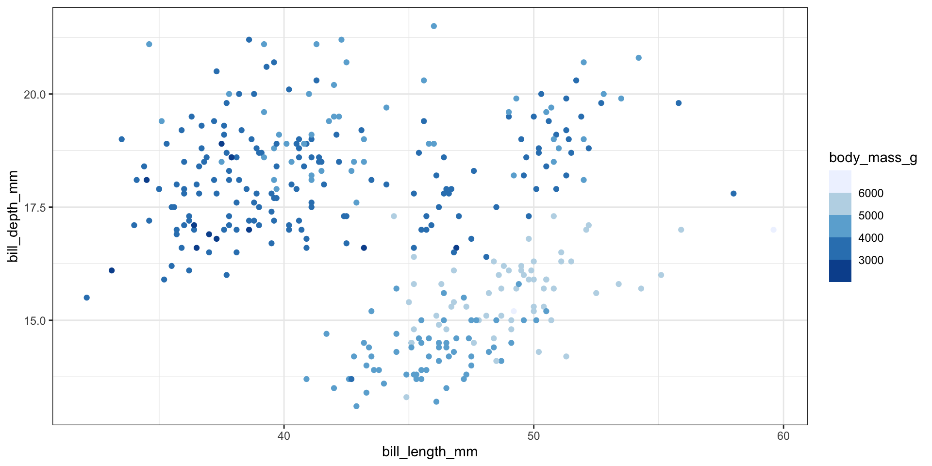
FAQ: Color Palettes
library (ggplot2); library (palmerpenguins)ggplot (penguins, aes (x= bill_length_mm, y= bill_depth_mm, color= body_mass_g)) + geom_point () + theme_bw () + scale_color_fermenter (type= "seq" ) # Binned
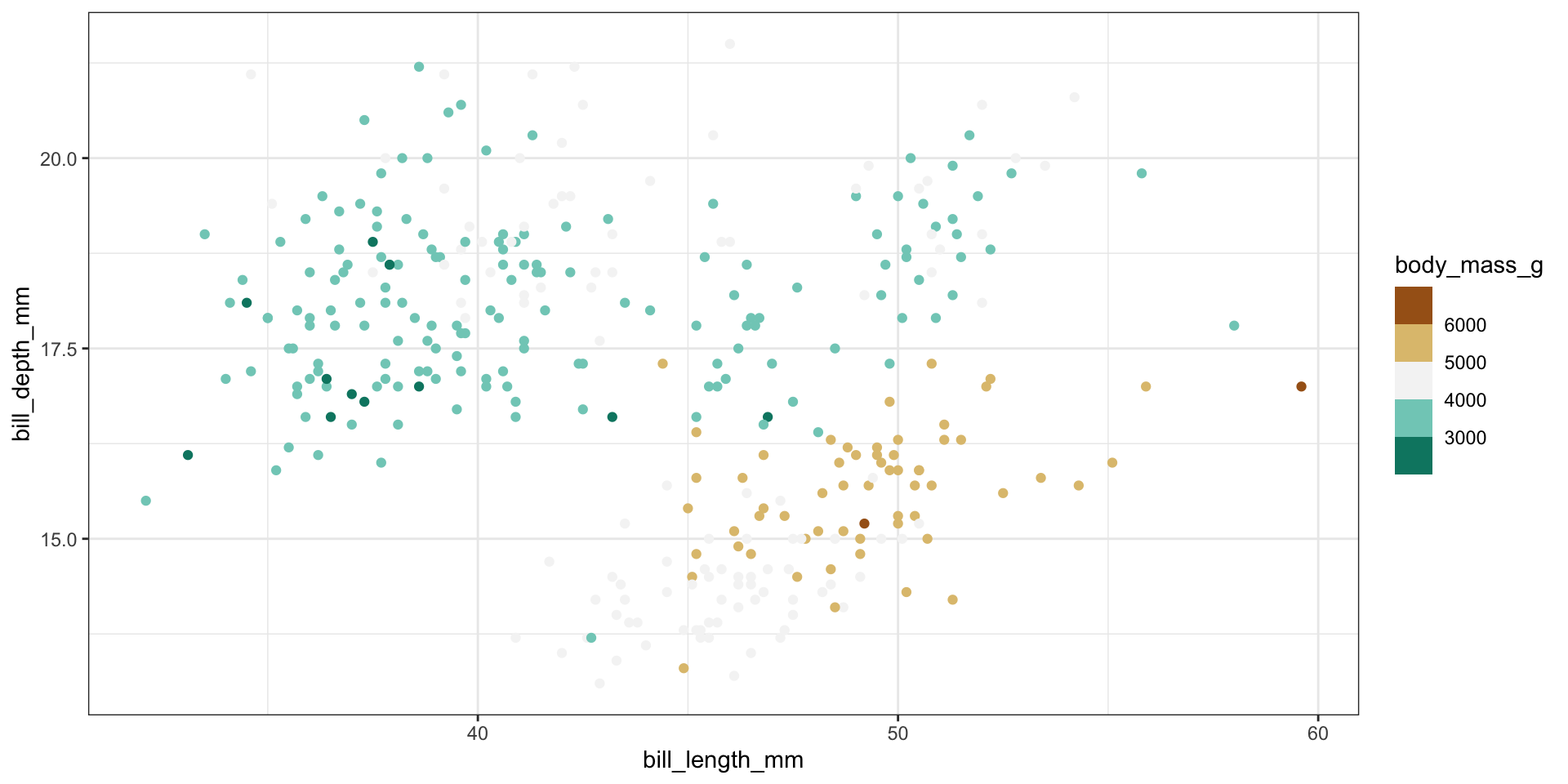
FAQ: Color Palettes
library (ggplot2); library (palmerpenguins)ggplot (penguins, aes (x= bill_length_mm, y= bill_depth_mm, color= body_mass_g)) + geom_point () + theme_bw () + scale_color_fermenter (type= "seq" ) # Binned + Sequential
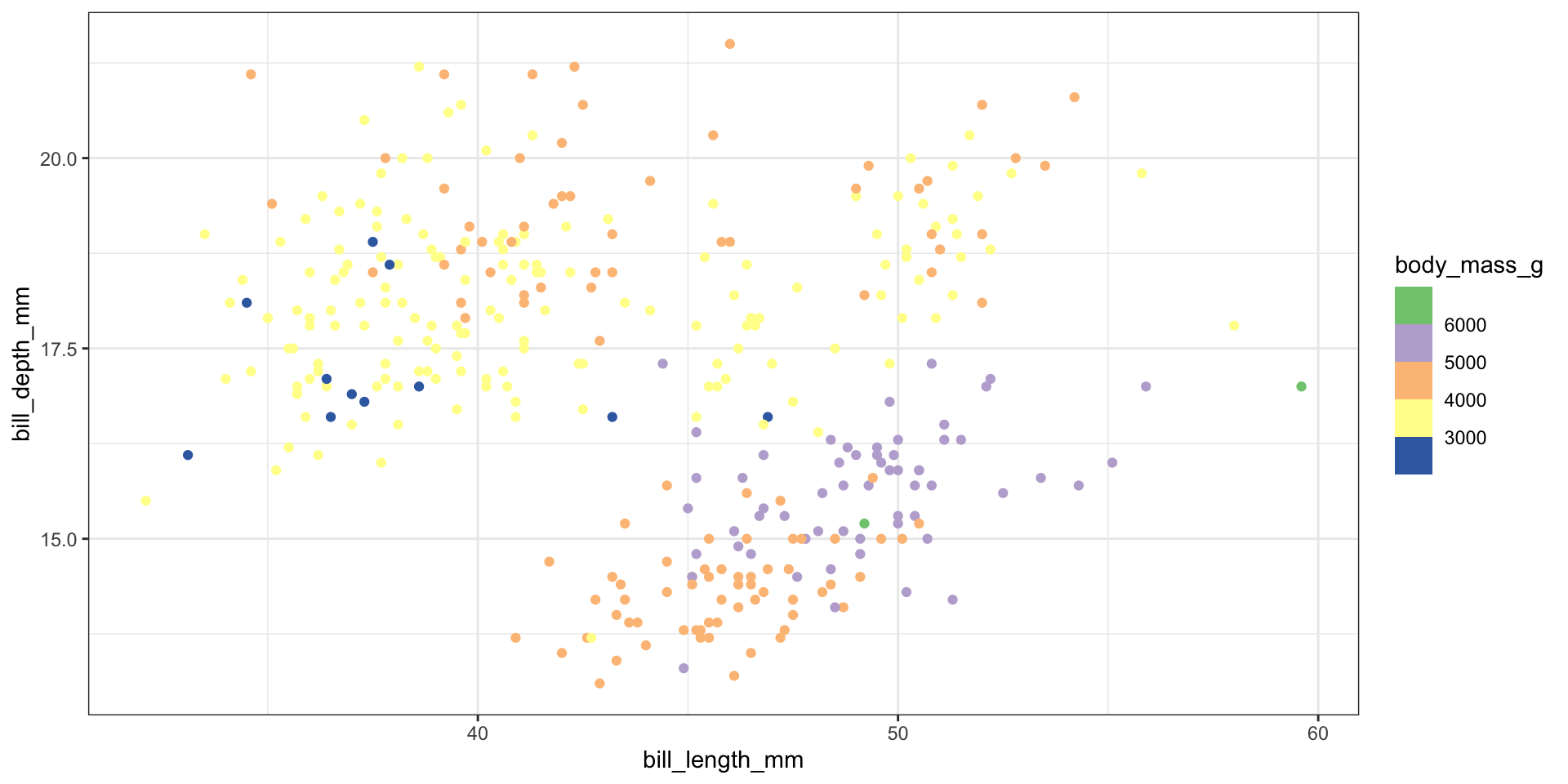
FAQ: Color Palettes
library (ggplot2); library (palmerpenguins)ggplot (penguins, aes (x= bill_length_mm, y= bill_depth_mm, color= body_mass_g)) + geom_point () + theme_bw () + scale_color_fermenter (type= "qual" ) # Binned + Qualitative
FAQ: Color Palettes
library (ggplot2); library (palmerpenguins)ggplot (penguins, aes (x= bill_length_mm, y= bill_depth_mm, color= body_mass_g)) + geom_point () + theme_bw () + scale_color_fermenter (type= "div" ) # Binned + Diverging
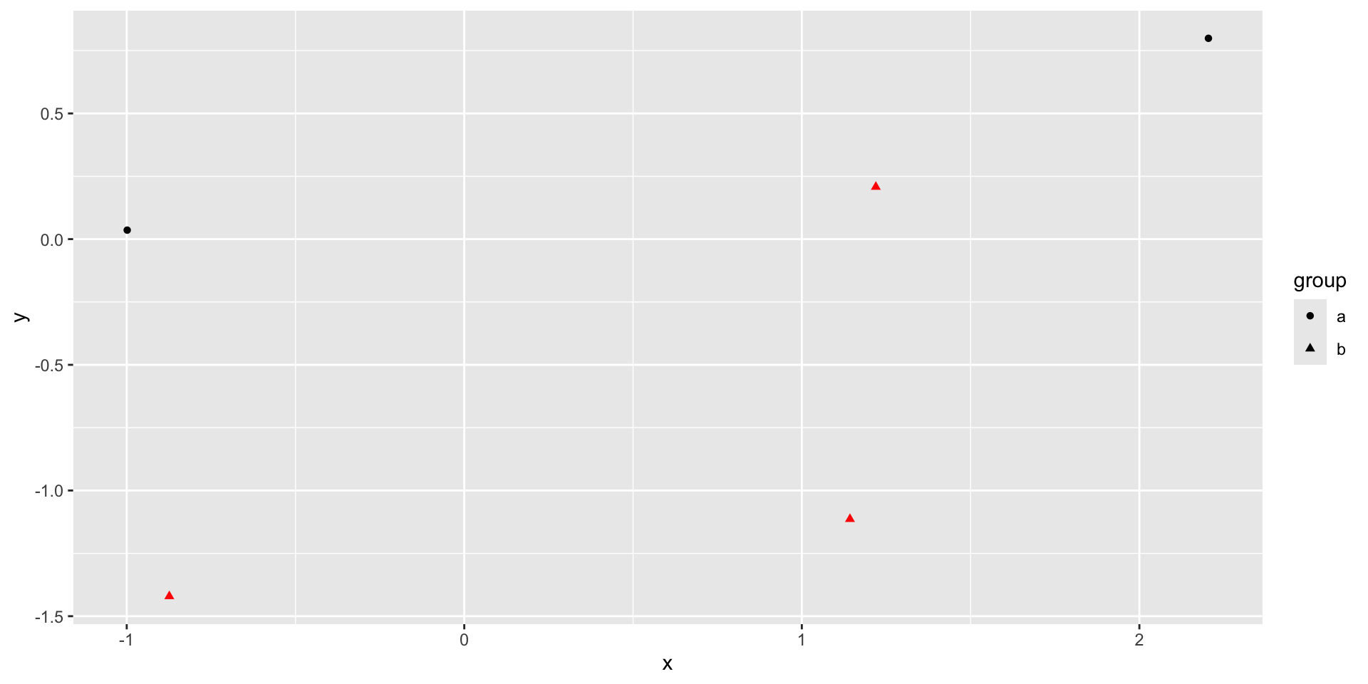
FAQ: How to “hard-code” colors
library (dplyr)<- data.frame (x = rnorm (5 ), y = rnorm (5 ), group = c ("a" , "a" , "b" , "b" , "b" ))|> group_by (group) |> mutate (n_count = n ()) |> ungroup () |> mutate (color = ifelse (n_count == max (n_count), "red" , "black" )) |> ggplot (aes (x= x, y= y, shape= group, color= color)) + geom_point () + scale_color_identity ()
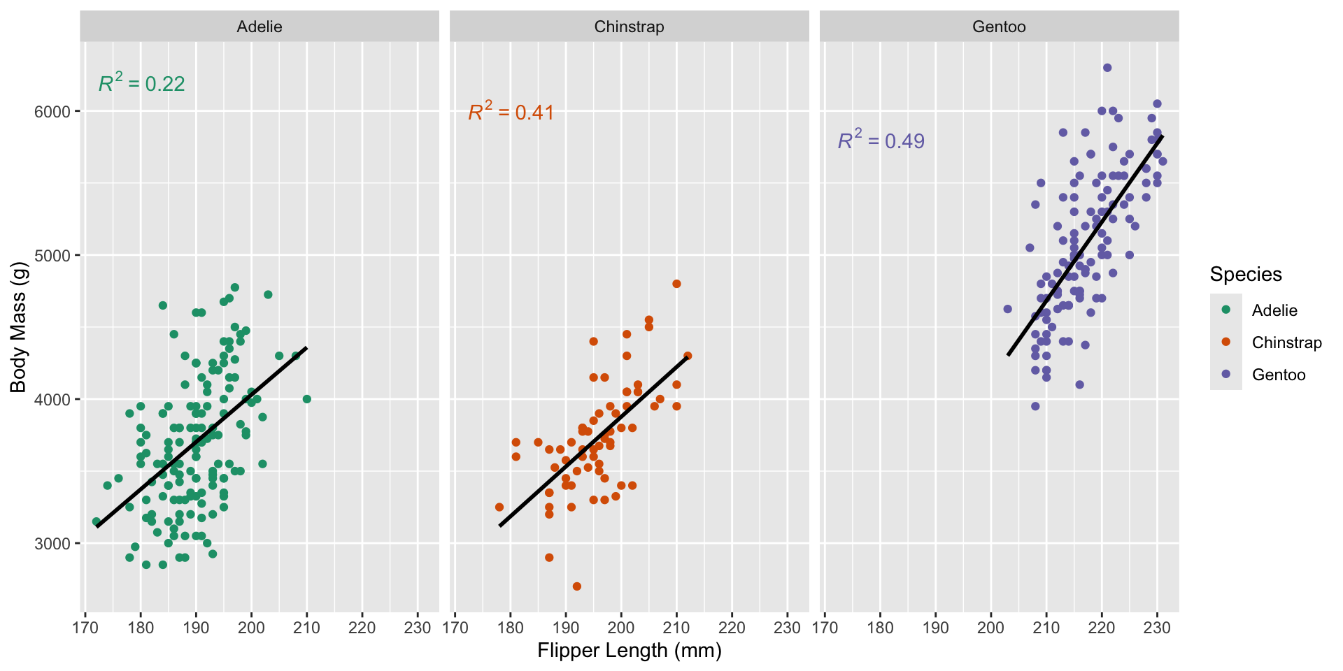
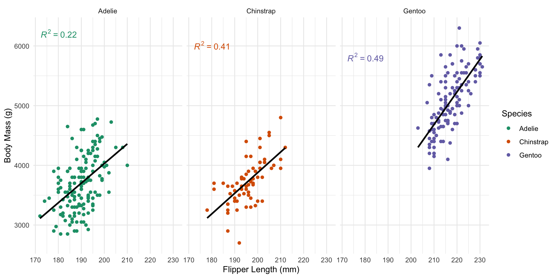
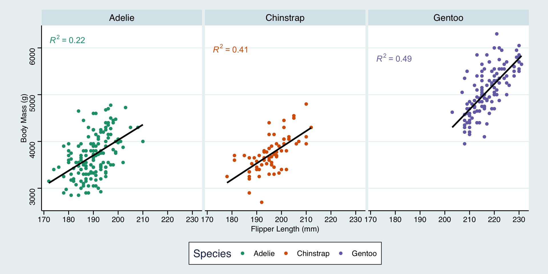
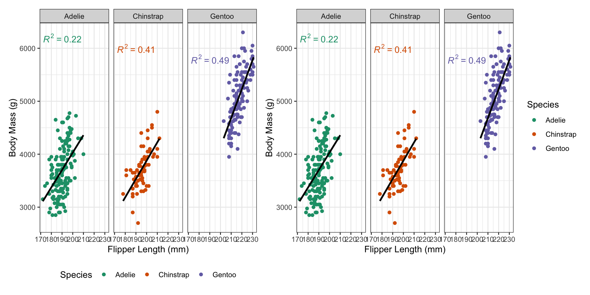
FAQ: How to Customize Themes
Built-in themes + ggthemes package:
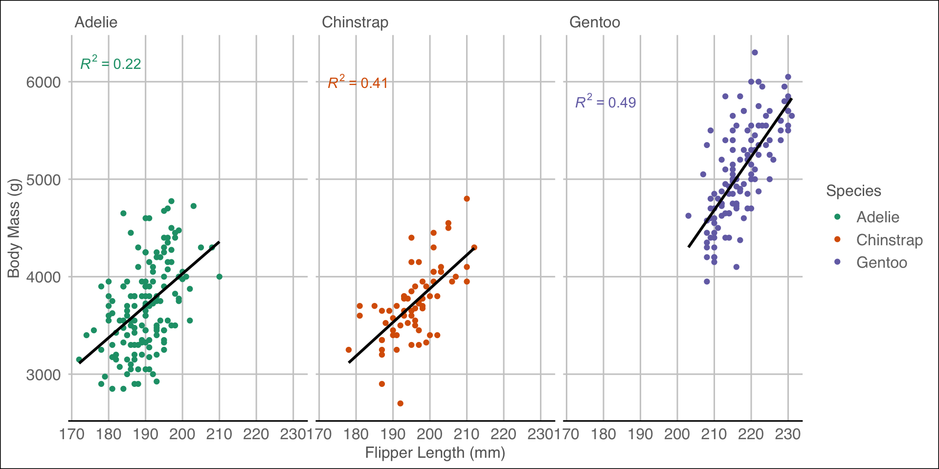
library (ggplot2); library (ggthemes); library (palmerpenguins); library (ggpmisc)<- ggplot (penguins, aes (x= flipper_length_mm, y= body_mass_g, color= species)) + geom_point () + stat_poly_line (se= FALSE , color= "black" ) + stat_poly_eq () + xlab ("Flipper Length (mm)" ) + ylab ("Body Mass (g)" ) + scale_color_brewer (type= "qual" , palette= 2 , name= "Species" ) + facet_wrap (~ species)
FAQ: Themes
Default theme (ggplot2::theme_grey()):
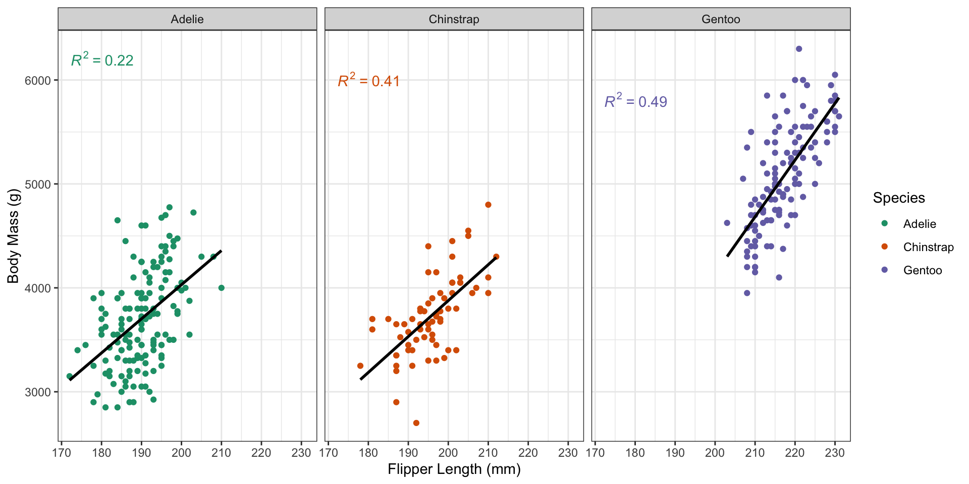
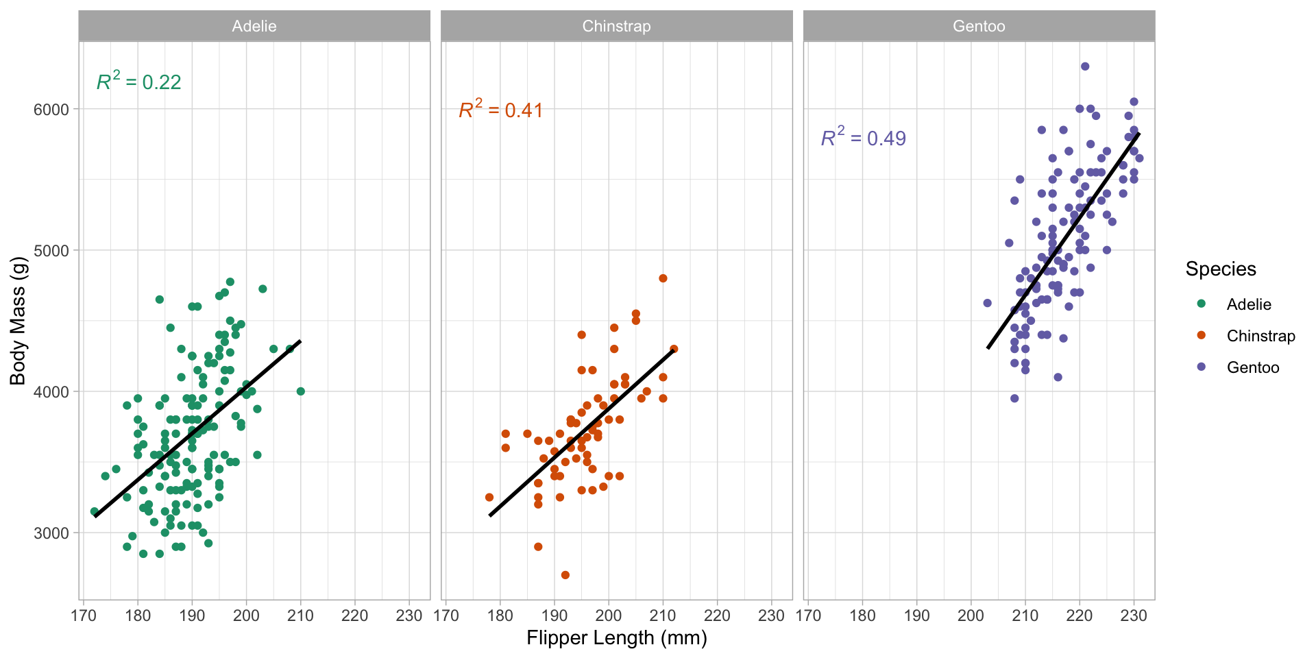
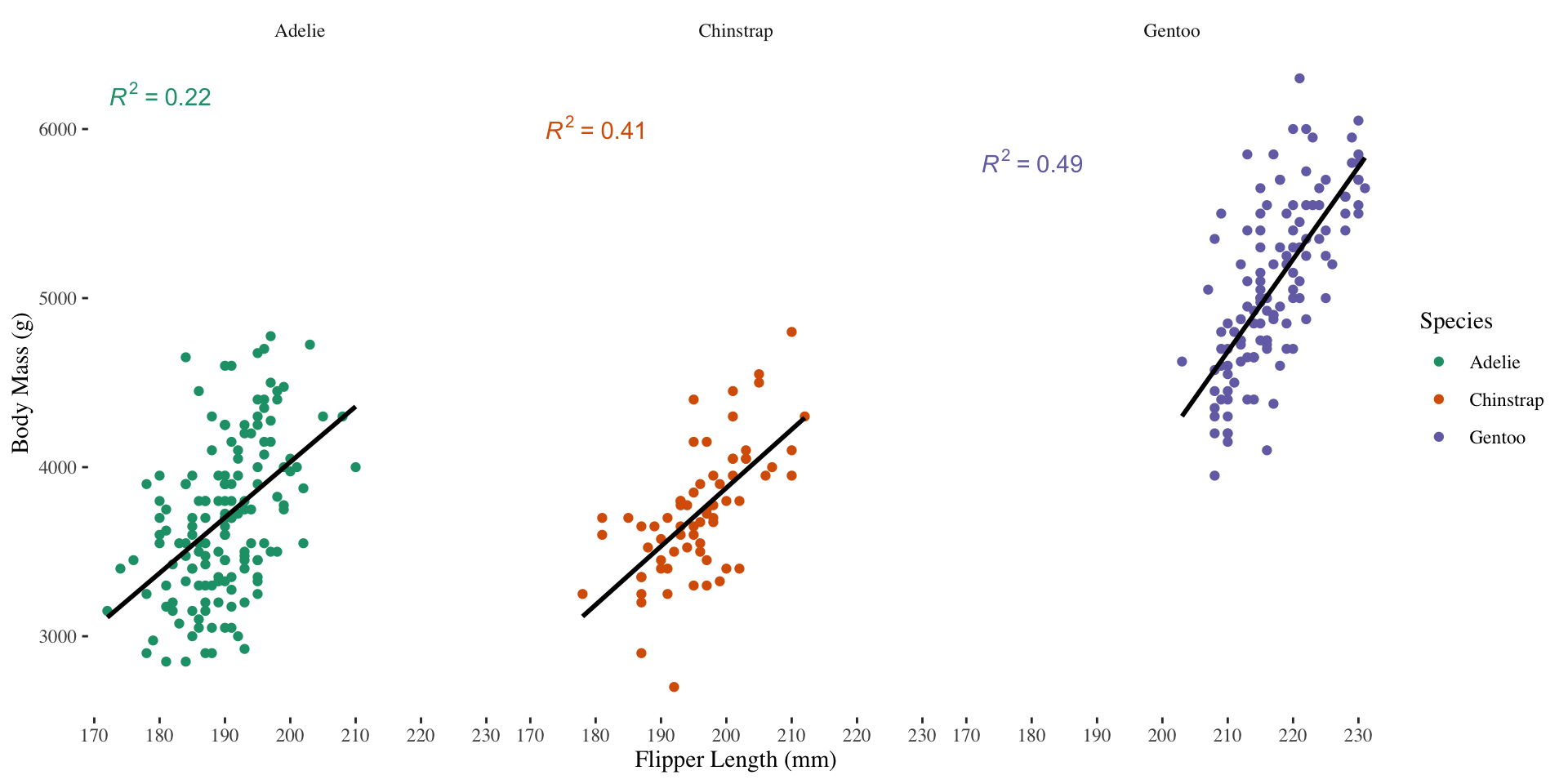
FAQ: Themes
Black and White theme (ggplot2::theme_bw()):
FAQ: Themes
Minimal theme (ggplot2::theme_minimal()):
FAQ: Themes
Light theme (ggplot2::theme_light()):
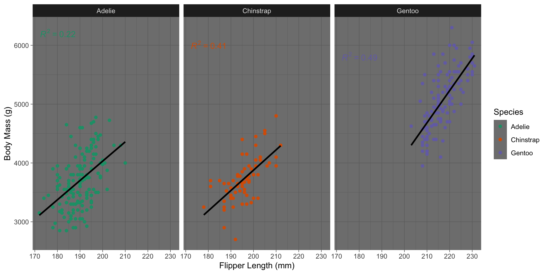
FAQ: Themes
Dark theme (ggplot2::theme_dark()):
FAQ: Themes
Excel theme (ggthemes::theme_excel()):
FAQ: Themes
Google Docs theme (ggthemes::theme_gdocs()):
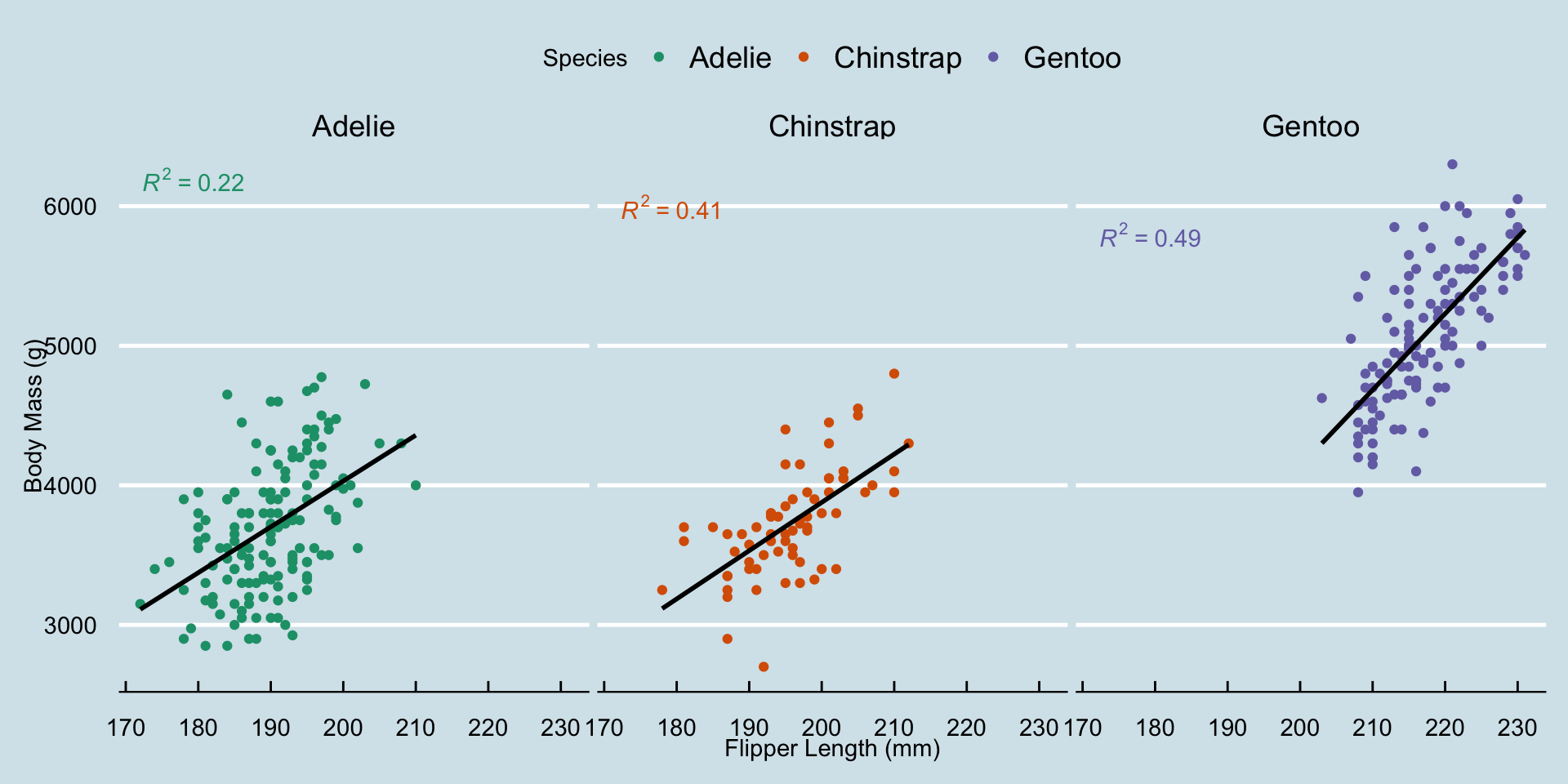
FAQ: Themes
The Economist theme (ggthemes::theme_economist()):
FAQ: Themes
The Economist theme (ggthemes::theme_economist()):
FAQ: Themes
Solarized theme (ggthemes::theme_solarized()):
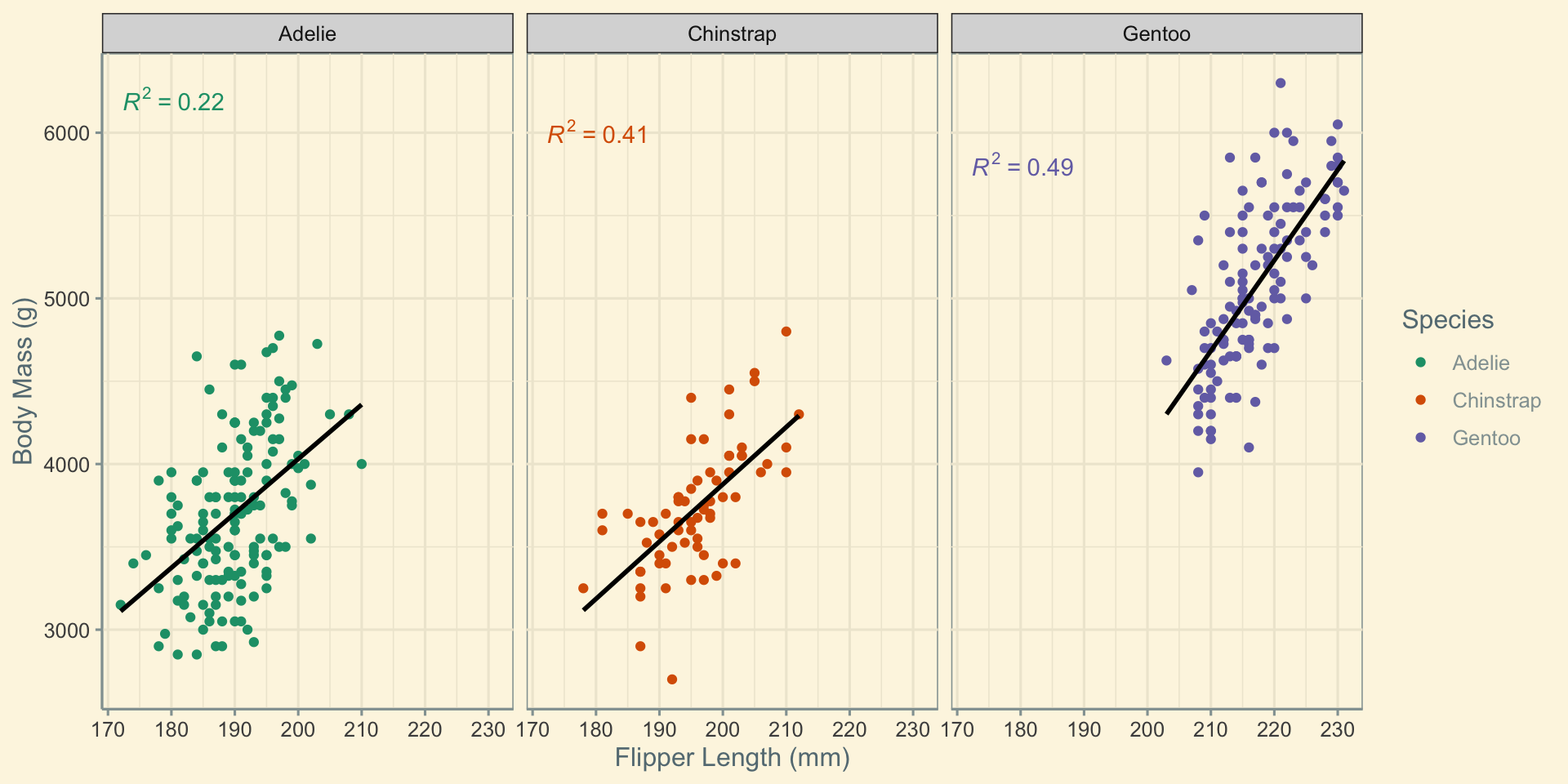
FAQ: Themes
Solarized2 theme (ggthemes::theme_solarized_2()):
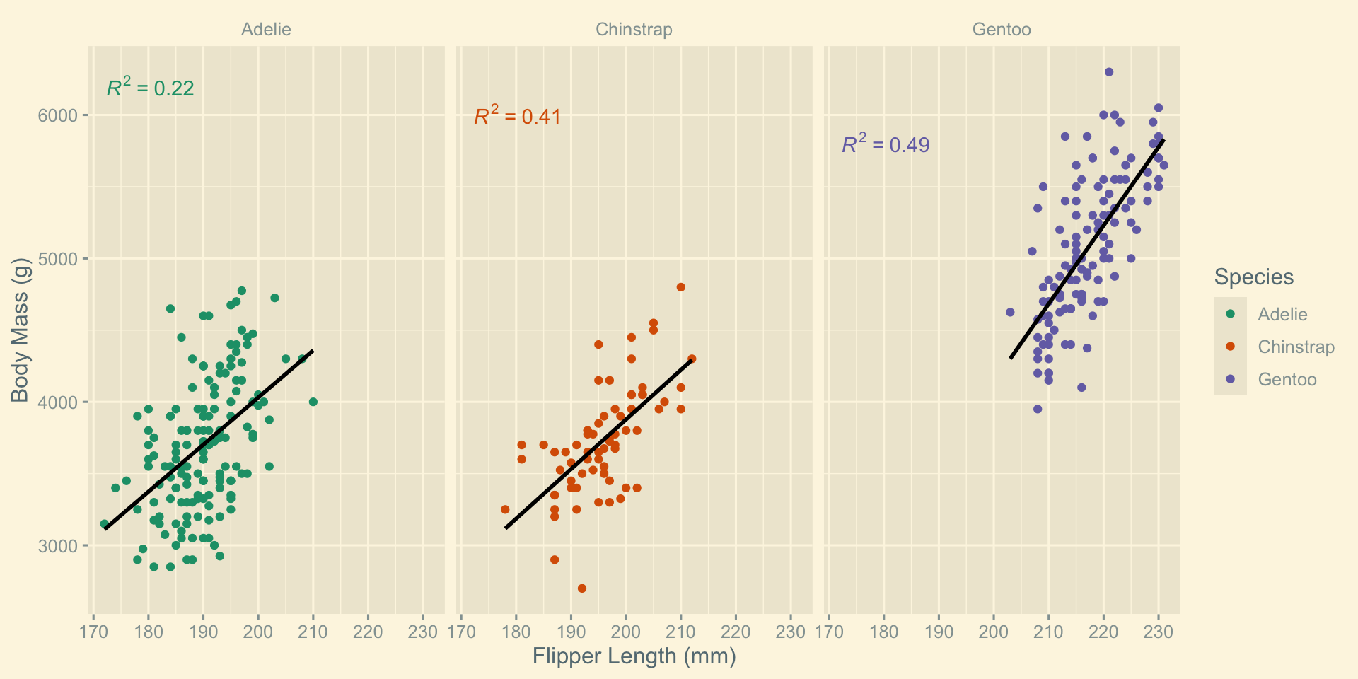
FAQ: Themes
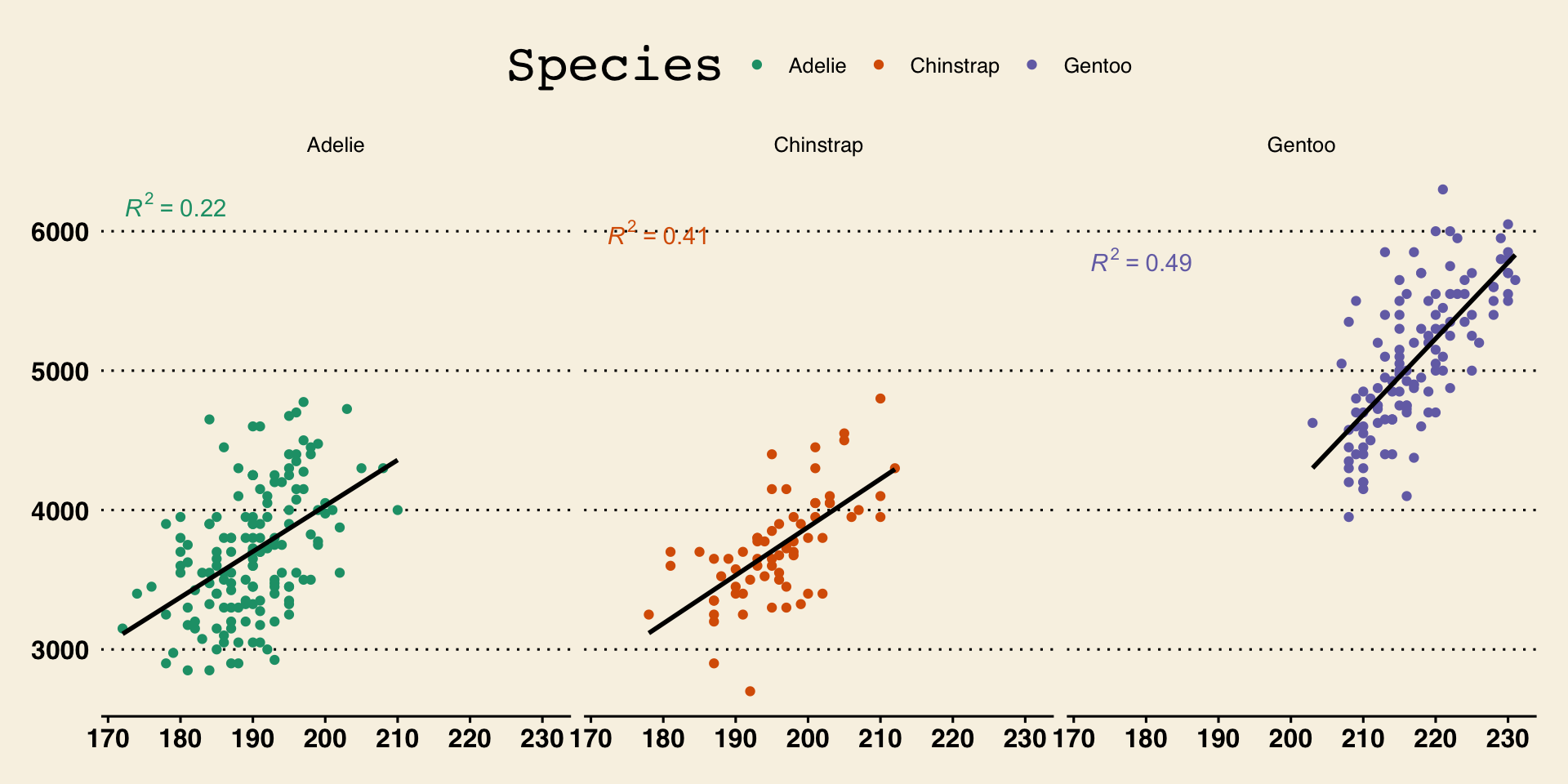
Stata theme (ggthemes::theme_stata()):
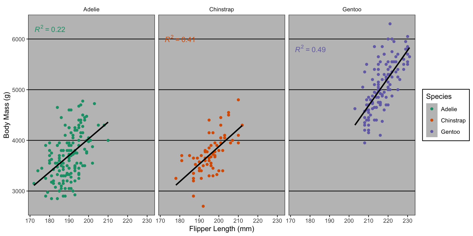
FAQ: Themes
Tufte theme (ggthemes::theme_tufte()):
FAQ: Themes
Wall Street Journal theme (ggthemes::theme_wsj()):
FAQ: Themes
Many more online:
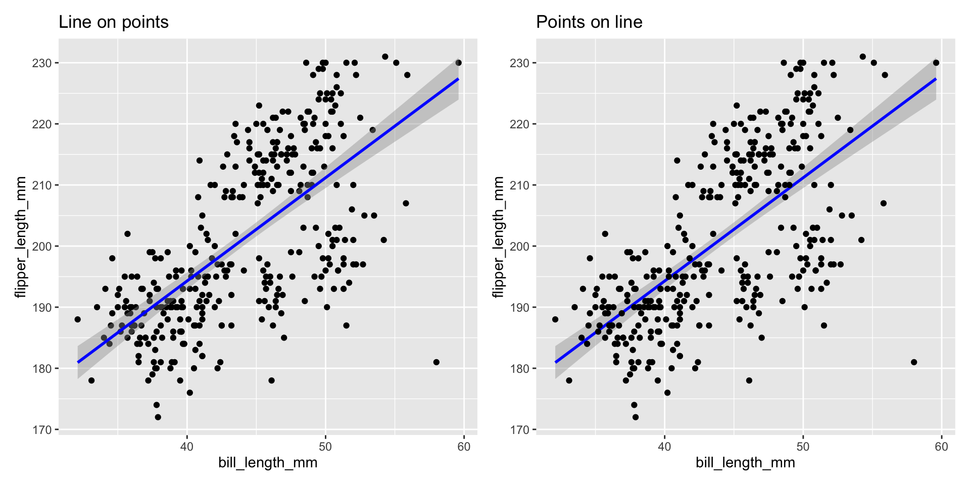
FAQ: Order of Layers
Order of layers technically matters, but the effect is small
<- ggplot (penguins, aes (x= bill_length_mm, y= flipper_length_mm)) + geom_point (color= "black" ) + geom_smooth (color= "blue" , method= "lm" ) + ggtitle ("Line on points" )<- ggplot (penguins, aes (x= bill_length_mm, y= flipper_length_mm)) + geom_smooth (color= "blue" , method= "lm" ) + geom_point (color= "black" ) + ggtitle ("Points on line" )+ p2
FAQ: Order of layers
Order matters more with theme. Adding a theme_*() will override any theme() customization you did:
<- p + theme_bw () + theme (legend.position= "bottom" )<- p + theme (legend.position= "bottom" ) + theme_bw () + p2
FAQ: stat_poly_{line,eq} vs geom_smooth
By default geom_smooth fits a generalized additive model (GAM)
ggpmisc::stat_poly_{line,eq} fit linear models, so they can expose more machinery.
What is a GAM?
Take 9890 with me (typically Spring semester) to find out!
Free Course: “GAMs in R” from Noam Ross
FAQ: Titles and Captions
ggplot () + labs (title= "Title" , subtitle= "Subtitle" , caption= "Caption" ,tag= "Tag" , alt= "Alt-Text" , alt_insight= "Alt-Insight" )
+ggtitle("text") is just shorthand for +labs(title="text")
FAQ: Relative Importance of Aesthetics
Perceptually:
Location > Color > Size > Shape
Humans are better at:
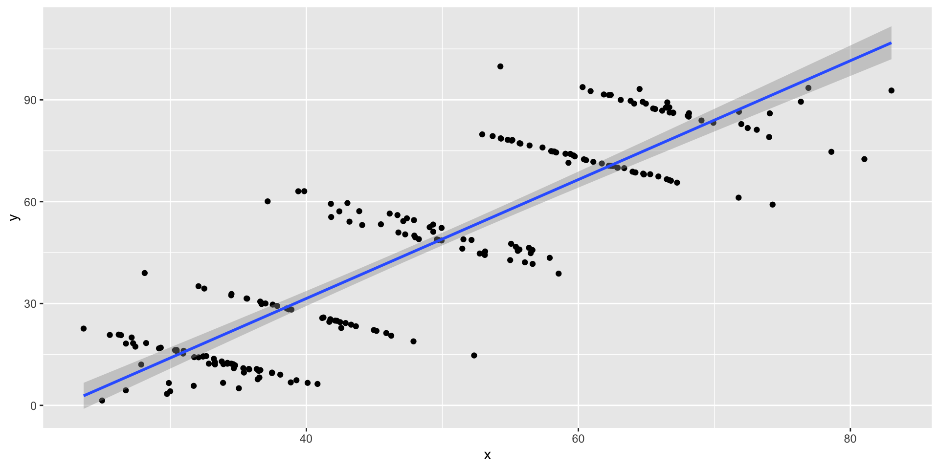
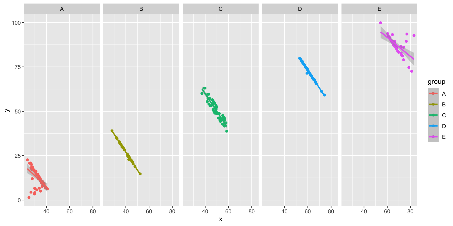
FAQ: When to Use Facets?
Facets are group_by for plots. Useful for
Distinguishing intra- vs inter-group trends
Avoiding overplotting
FAQ: Simpson’s Paradox
FAQ: Simpson’s Paradox
FAQ: UCB Graduate Admissions
1973: UC Berkeley was concerned about bias in Grad School Admissions
Higher fraction of men admitted than women
Bickel, Hammell, O’Connell asked to study
When they try to find the source of this bias, there is none!
Each department admits women at a higher rate than men
Women applied to more selective programs at a higher rate
This phenomenon occurs throughout the social sciences: the best doctors have the worst patient outcomes
BHO note:
Women are shunted by their socialization and education toward fields of graduate study that are generally more crowded, less productive of completed degrees, and less well funded, and that frequently offer poorer professional employment prospects.
FAQ: Twin Axes Plots
How can I implement a dual (twin) axis plot in ggplot2?
Disfavored. But if you must …
sec.axis
Doesn’t allow arbitrary secondary axes; allows transformed axes (e.g., Celsius and Fahrenheit)
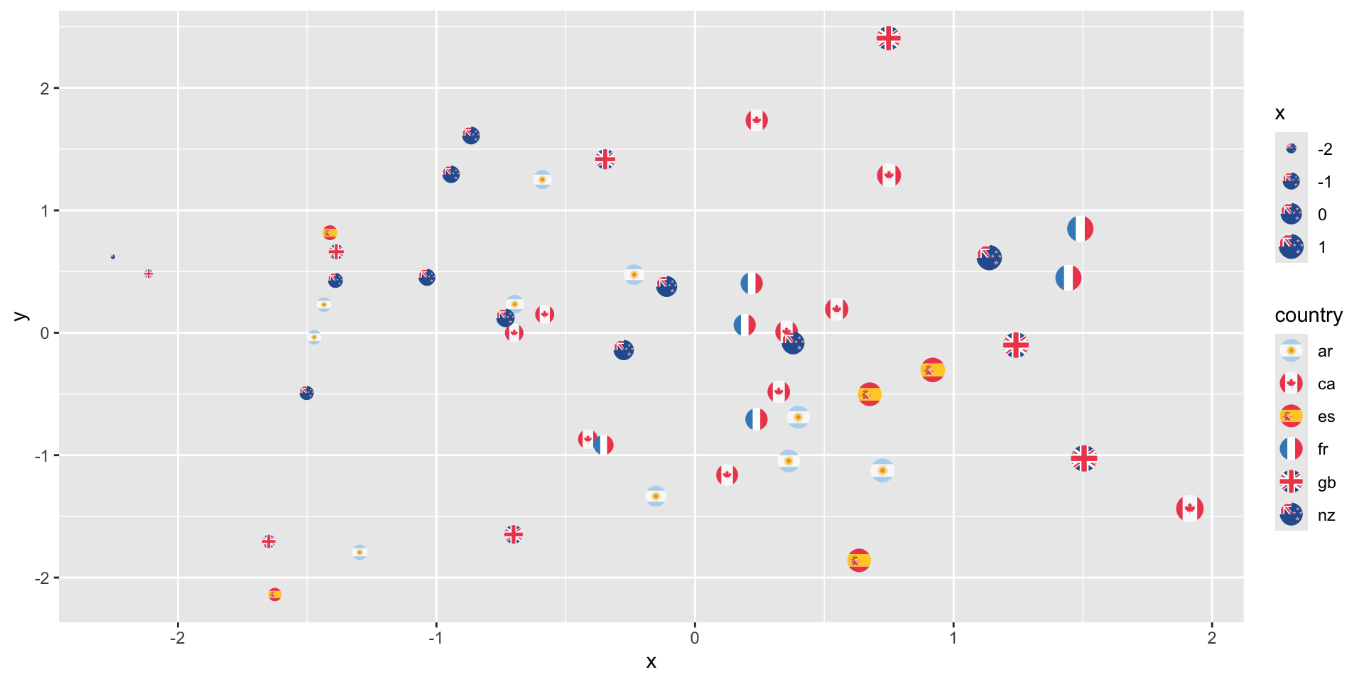
FAQ: Embedding images in ggplot
See the ggimage or ggflags package for images as “points”:
#devtools::install_github("jimjam-slam/ggflags"); library (ggflags)<- data.frame (x= rnorm (50 ), y= rnorm (50 ), country= sample (c ("ar" ,"fr" , "nz" , "gb" , "es" , "ca" ), 50 , TRUE ), stringsAsFactors = FALSE )ggplot (d, aes (x= x, y= y, country= country, size= x)) + geom_flag () + scale_country ()
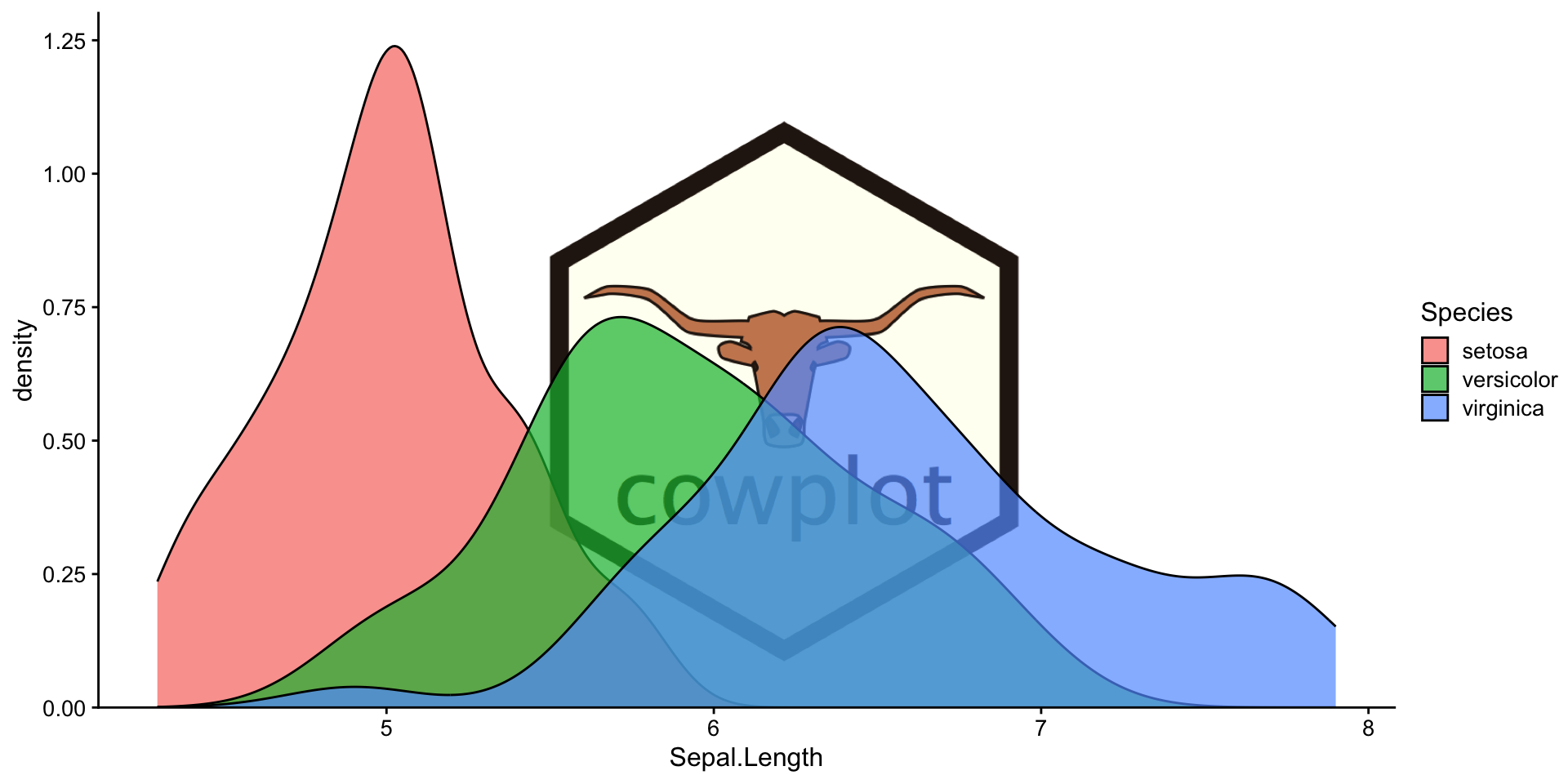
FAQ: Embedding Images
See cowplot::draw_image() for image background:
library (cowplot)<- ggplot (iris, aes (x = Sepal.Length, fill = Species)) + geom_density (alpha = 0.7 ) + scale_y_continuous (expand = expansion (mult = c (0 , 0.05 ))) + theme_half_open (12 )<- system.file ("extdata" , "logo.png" , package = "cowplot" )ggdraw () + draw_image (scale = .7 + draw_plot (p)