Software Tools for Data Analysis
STA 9750
Michael Weylandt
Week 10 – Tuesday 2026-04-21
Last Updated: 2026-04-21

STA 9750 Week 10

Today: Lecture #08: Advanced ggplot2 – maps, interactivity, animation

These slides can be found online at:

https://michael-weylandt.com/STA9750/slides/slides10.html

In-class activities can be found at:

https://michael-weylandt.com/STA9750/labs/lab08.html

Upcoming TODO

Upcoming student responsibilities:

Date	Time	Details
2026-04-23	6:00pm ET	Pre-Assignment #11 Due
2026-04-24	11:59pm ET	Mini-Project #03 Due
2026-04-30	6:00pm ET	Pre-Assignment #12 Due
2026-05-03	11:59pm ET	Mini-Project Peer Feedback #03 Due
2026-05-07	6:00pm ET	Final Project Presentation Slides Due
2026-05-14	6:00pm ET	Pre-Assignment #14 Due
2026-05-15	11:59pm ET	Mini-Project #04 Due

STA 9750 Week 10

Today: Lecture #08: Advanced ggplot2 – maps, interactivity, animation

• Communicating Results (quarto) ✅
• R Basics ✅
• Data Manipulation in R ✅
• Data Visualization in R ⬅️
  • Static Plots ✅
  • Interactivity, Maps, Animated Plots ⬅️
• Getting Data into R
• Statistical Modeling in R

Today

Today

• Course Administration
• Review Exercise
• Advanced ggplot2
  • Spatial Data (Maps)
  • Animation
  • Interactivity
• Wrap-Up
  • Life Tip of the Day

Administrative Business

STA 9750 Mini-Projects

• Mini-Project #01 ✅ (2026-03-13 at 11:59pm ET)
• Mini-Project #02 ✅ (2026-04-03 at 11:59pm ET)
• Mini-Project #03 (2026-04-24 at 11:59pm ET)
  • Submission ⬅️
  • Peer Feedback
• Mini-Project #04 (2026-05-15 at 11:59pm ET)

Mini-Project #03

MP#03 - Who Goes There? US Internal Migration and Implications for Congressional Reapportionment

Due 2026-04-24 at 11:59pm ET

Topics covered:

• Data Import
  • Package Usage
  • Static Files
  • API Calls
• Advanced Data Manipulation
• Spatial Data Visualization (Optional)

Future Mini-Projects

MP#04 - Going for the Gold

Due 2026-05-15 at 11:59pm ET

Topics covered:

• Data Import
  • HTTP Requests
  • HTML Scraping (Tabular)
  • Text Processing
• \(t\)-tests
• Putting Everything Together

Course Support

• Synchronous: MW Office Hours 2x / week:
  • Wednesdays 5pm in-person
  • Thursdays 5pm on Zoom
• Asynchronous: Piazza

Course Project

Course Project should be your main focus for rest of course

• But you still need to do mini-projects and pre-assignments(!)

Course Project

Final submissions:

• Detailed rubrics for group report + individual report
  • Final Group Report
  • Final Individual Report

Notes added on integration of SQs and strategies for estimating causal effects. Ask questions! I’m happy to fill these out further.

Review Exercise

SSA Registered Births

Time series data of babies born and registered with the Social Security Administration (previously in Lab #05)

Rows: 7,305
Columns: 7
$ year        <dbl> 1969, 1969, 1969, 1969, 1969, 1969, 1969, 1969, 1969, 1969…
$ month       <dbl> 1, 1, 1, 1, 1, 1, 1, 1, 1, 1, 1, 1, 1, 1, 1, 1, 1, 1, 1, 1…
$ day         <dbl> 1, 2, 3, 4, 5, 6, 7, 8, 9, 10, 11, 12, 13, 14, 15, 16, 17,…
$ births      <dbl> 8486, 9002, 9542, 8960, 8390, 9560, 9738, 9734, 9434, 1004…
$ day_of_year <dbl> 1, 2, 3, 4, 5, 6, 7, 8, 9, 10, 11, 12, 13, 14, 15, 16, 17,…
$ day_of_week <dbl> 3, 4, 5, 6, 7, 1, 2, 3, 4, 5, 6, 7, 1, 2, 3, 4, 5, 6, 7, 1…
$ id          <dbl> 1, 2, 3, 4, 5, 6, 7, 8, 9, 10, 11, 12, 13, 14, 15, 16, 17,…

SSA Registered Births

Practice visualization:

1. Are there months with more births?
2. Are there days of the week with more births?
3. Is there a long-term trend in births?

See Lab #08 for details.

Breakout Rooms

Breakout Room	Team
1	Maniac Braniacs (HHS+KK+FC+DN)
2	Water Benders (JE+JABB+MTP+JA+AS)
3	3-1-Fun! (XC+ML+ER+RJSN)
4	Emissions Impossible (LR+MOG+APTL)
5	Inspector Gadget (MUO+KN+CM+ID+KM)

Review activities from today’s lab

Advanced ggplot2

Spatial Data

Maps are more interesting than you think!

• The world isn’t flat!

This can get intense, but we will get by with simple features (sf)

Map Projections

WGS 84

WGS 84 is a robust and widely-used way of creating maps from 3D coordinates.

• Good default
• Convert existing sf using sf::st_transform(4326)

Not universal!

sf Package

The sf package provides tools for dealing with spatial data:

• st_read for reading geojson or shp files
• st_join for combining spatial data
• Integrates with ggplot2::geom_sf() for plotting

sf Objects

sf object - data.frame with additional geometry information

library(sf); library(tidyverse)
nc <- st_read(system.file("shape/nc.shp", package="sf"))

Reading layer `nc' from data source 
  `/Library/Frameworks/R.framework/Versions/4.5-arm64/Resources/library/sf/shape/nc.shp' 
  using driver `ESRI Shapefile'
Simple feature collection with 100 features and 14 fields
Geometry type: MULTIPOLYGON
Dimension:     XY
Bounding box:  xmin: -84.32385 ymin: 33.88199 xmax: -75.45698 ymax: 36.58965
Geodetic CRS:  NAD27

glimpse(nc)

Rows: 100
Columns: 15
$ AREA      <dbl> 0.114, 0.061, 0.143, 0.070, 0.153, 0.097, 0.062, 0.091, 0.11…
$ PERIMETER <dbl> 1.442, 1.231, 1.630, 2.968, 2.206, 1.670, 1.547, 1.284, 1.42…
$ CNTY_     <dbl> 1825, 1827, 1828, 1831, 1832, 1833, 1834, 1835, 1836, 1837, …
$ CNTY_ID   <dbl> 1825, 1827, 1828, 1831, 1832, 1833, 1834, 1835, 1836, 1837, …
$ NAME      <chr> "Ashe", "Alleghany", "Surry", "Currituck", "Northampton", "H…
$ FIPS      <chr> "37009", "37005", "37171", "37053", "37131", "37091", "37029…
$ FIPSNO    <dbl> 37009, 37005, 37171, 37053, 37131, 37091, 37029, 37073, 3718…
$ CRESS_ID  <int> 5, 3, 86, 27, 66, 46, 15, 37, 93, 85, 17, 79, 39, 73, 91, 42…
$ BIR74     <dbl> 1091, 487, 3188, 508, 1421, 1452, 286, 420, 968, 1612, 1035,…
$ SID74     <dbl> 1, 0, 5, 1, 9, 7, 0, 0, 4, 1, 2, 16, 4, 4, 4, 18, 3, 4, 1, 1…
$ NWBIR74   <dbl> 10, 10, 208, 123, 1066, 954, 115, 254, 748, 160, 550, 1243, …
$ BIR79     <dbl> 1364, 542, 3616, 830, 1606, 1838, 350, 594, 1190, 2038, 1253…
$ SID79     <dbl> 0, 3, 6, 2, 3, 5, 2, 2, 2, 5, 2, 5, 4, 4, 6, 17, 4, 7, 1, 0,…
$ NWBIR79   <dbl> 19, 12, 260, 145, 1197, 1237, 139, 371, 844, 176, 597, 1369,…
$ geometry  <MULTIPOLYGON [°]> MULTIPOLYGON (((-81.47276 3..., MULTIPOLYGON ((…

Chloropleths

A map whose fill depends on the value of interest is called a chloropleth:

ggplot(nc, aes(fill=BIR79 / BIR74 - 1, geometry=geometry)) + 
  geom_sf() + 
  guides(fill="none") + 
  ggtitle("% Change in Number of Children Born Per Year 1974-1979")

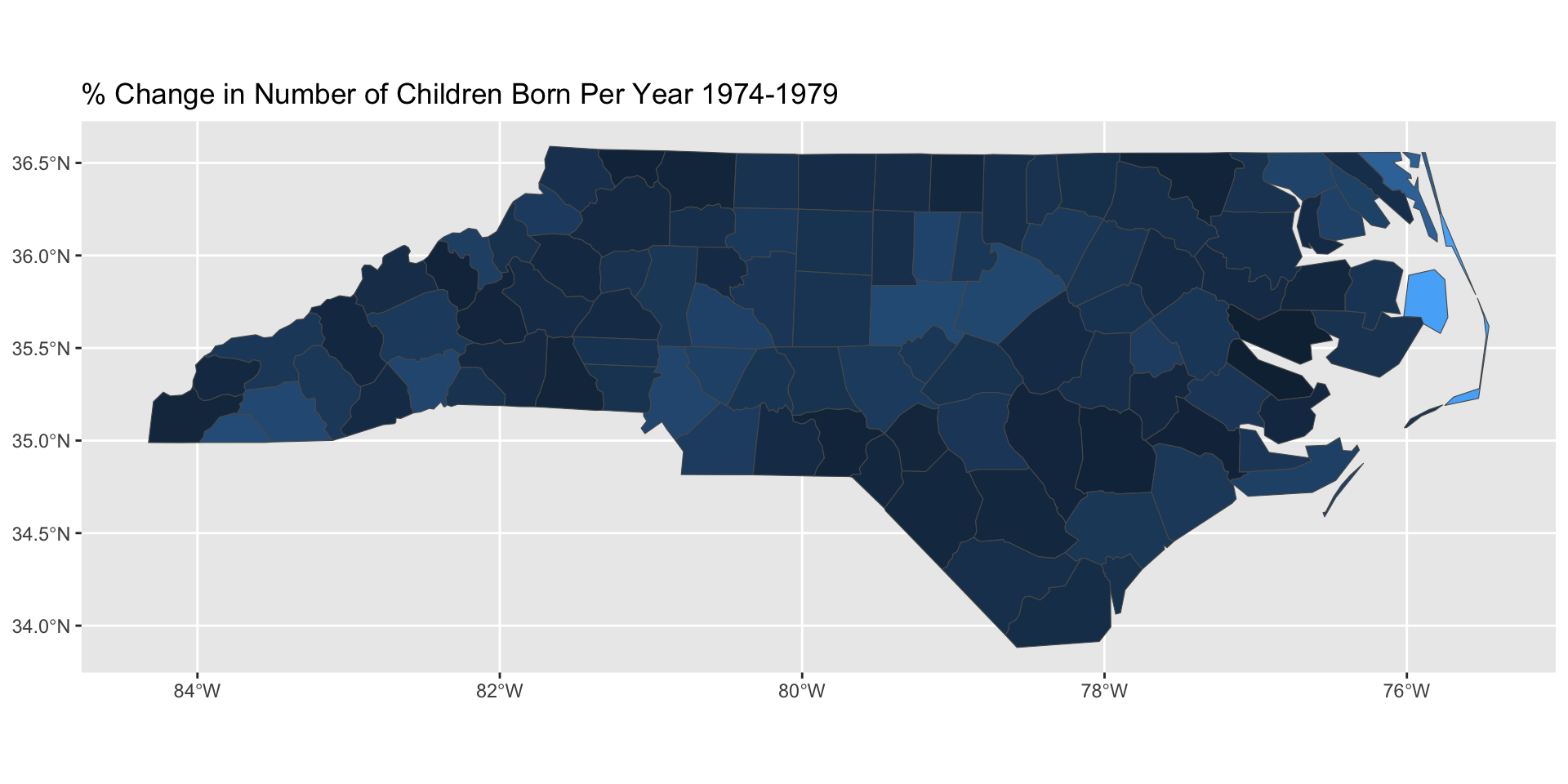
Integrates well with ggplot2:

• geom_sf knows how to handle geometries
• other features all work as expected (fill, animation, legends, etc.)

Breakout Exercises

Two sets of spatial exercises:

• Chloropleths
• Cartograms

Spatial Data in Lab #08

Animation

Animated Graphics

gganimate is the de facto standard for animated ggplot2:

• Make a bunch of png files
• Combine into a gif

Most commonly: +transition_time(VARIABLE)

NB: Unlike facet_wrap, no ~ before VARIABLE

transition_*() functions

Animation is implemented via a new plot element: transition_*():

library(gganimate)
ggplot(births, aes(x=day_of_year, y=births)) +
  geom_line() + 
  transition_time(year)

transition_*() functions

Add a title to indicate time being shown:

library(gganimate)
ggplot(births, aes(x=day_of_year, y=births)) +
  geom_line() + 
  transition_time(year) + ggtitle("Year: {frame_time}")

transition_*() functions

gganimate “tweens” (interpolates) between frames for smoothness - works best for continuous time data.

It’s a bit weird here and we might prefer a more discrete interpolation:

library(gganimate)
ggplot(births, aes(x=day_of_year, y=births)) +
  geom_line() + 
  transition_states(year) + ggtitle("Year: {closest_state}")

Easing

Use the ease_ functions (or enter_()/exit_*() separately) for finer control:

ggplot(births, aes(x=day_of_year, y=births, group=year)) +
  geom_line() + transition_states(year, transition_length = 4, state_length=1) + 
  ggtitle("Year: {closest_state}") + enter_grow() + exit_fade()

Grouping

The group variable is used to determine whether something is permanent over time.

penguins |> drop_na() |>
  ggplot(aes(x = bill_dep, y = body_mass)) +
  geom_point() + ggtitle("{frame_time}") + 
  transition_time(year)

Bad! Doesn’t make sense to interpolate penguins

Grouping

penguins |> drop_na() |>
  ggplot(aes(x = bill_dep, y = body_mass, group=year)) +
  geom_point() + ggtitle("{floor(frame_time)}") + 
  transition_time(year)

See gganimate Getting Started Documentation for more

Breakout Exercises

Animation exercises:

• gapminder data
• How has the world gotten healthier and richer over the past century?

Animated Visualizations in Lab #08

Animated Graphics

When it works, gganimate is great

• PITA when external software is busted

Alternatives:

• Facet plots
• Split facets over pages and scroll quickly: ggforce::facet_wrap_paginate()
• Interactivity with autoplay

Caution: think about how transitions should be structured

Interactivity

Interactivity

The ggiraph package provides for interactive ggplot2

Alternatives

The plotly package provides a ggplotly() function which works similarly.

Advantages:

• Has a more sophisticated “time change” interactivity

Disadvantages

• Doesn’t support all of ggplot2

Alternatives

Example of ggplotly - frame gives rise to a time slider:

library(plotly)
G <- ggplot(births, aes(x=day_of_year, y=births, frame=year)) +
  geom_point() + geom_line() + theme_bw()
ggplotly(G)

Shiny

Plotting FAQs

ggplot2 & Pie Charts

Why do Pie Charts have a bad reputation?

• Use of area and angle over length: less accurate perception
• Depends on fill to convey category - limited categories

But primarily - “insider smugness” and hate of Excel

ggplot2 Plot Type Choice

For me:

• Exploratory mode:
  • Simple: line, scatter, bar, frequency
• Publication mode:
  • Very context specific
  • “Simplicity” / “Elegance” depend on audience expectations

ggplot2 Font Sizing

Theme machinery!

ggplot(iris, aes(x=Sepal.Length, y=Sepal.Width)) + 
    geom_point() + theme(axis.text = element_text(size=24))

Overplotting / ScatterBlobs

Student asked about “scatterblobs” - typo(?) but I love it!

• Density based plotting: hexbins, histograms, rugplots
• Data reduction: summarization or sub-sampling

Optimizing ggplot2 Performance

Active project of ggplot2 team - not much you can do

Practical advice:

• Plot less (see previous slide)
• Take advantage of quarto Caching

ggplot2 Beyond Scatter and Line

Some favorite semi-advanced plot types:

• Violin plots: combination of boxplot and histogram
• Ridgelines
• Beeswarms

Deep rabbit hole

ggplot2 + High-Dimensional Data

High-dimensional data: measure many variables per observation (“wide”)

High-dimensional data is hard to visualize

Approaches:

• Pair plots for “moderate” HDD
• PCA (or similar dimension reduction. Take 9890!)

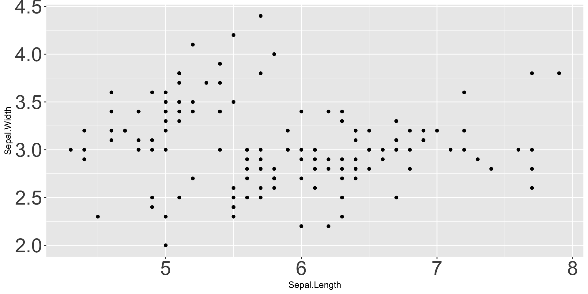
Custom ggplot2 Theme

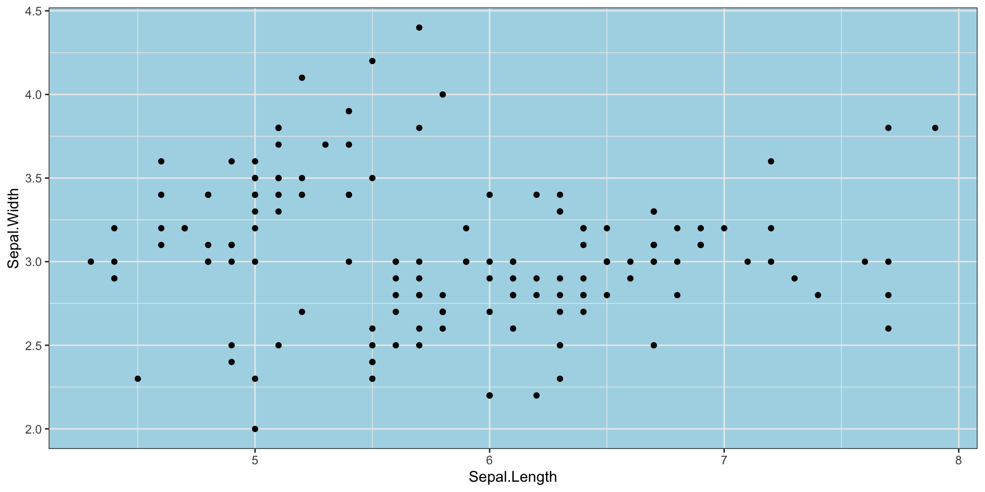
my_theme <- theme_bw() + theme(panel.background = element_rect(fill = 'lightblue'))
ggplot(iris, aes(x=Sepal.Length, y = Sepal.Width)) + geom_point() + my_theme

Advanced:

• theme_set() - change ggplot2 defaults
• .Rprofile - set code to run every time you start R

ggplot2 - When Not to Use

ggplot2 is designed to make good statistical graphics. Sub-par for:

• Very advanced interactivity (unless combined with shiny or custom JS)
• Really big data
• Hardcore customization / “infographics”

git WTF

Reference: Happy Git with R

Wrap-Up

Review

Advanced ggplot2:

• ggplot2 as a platform for powerful extensions
• Spatial data: sf
• Animation: gganimate
• Interactivity: ggiraph, shiny

Wrap-Up

Orientation

• Communicating Results (quarto) ✅
• R Basics ✅
• Data Manipulation in R ✅
• Data Visualization in R ✅
• Getting Data into R ⬅️
  • Files and APIs ✅
  • Web Scraping [Thursday]
  • Cleaning and Processing Text
• Statistical Modeling in R

Musical Treat