install.packages("styler")STA 9750 Lecture #1 In-Class Activity: Rev your Engines! Setting-Up R and RStudio
Class #01: Thursday January 29, 2026 (Lecture #01: Course Overview and Key Infrastructure)
Slides
Welcome!
Topics:
- Installing
RandRStudio - Installing
git - Getting Started on
GitHub - Basic Principles of “Clean Code”
R and RStudio
The primary programming language used in this course is R, one of the two most popular languages used in data science. R, like its predecessor the S language, is optimized for interactive, data-analytic work, in contrast with python, which is optimized for general purpose computing.
R is a programming language and runtime; we will supplement it with RStudio, an Integrated Development Environment or, less formally, an editor. RStudio is the software where you will write the code and then the R runtime will execute it.
R
Students should first install R from https://cloud.r-project.org/.
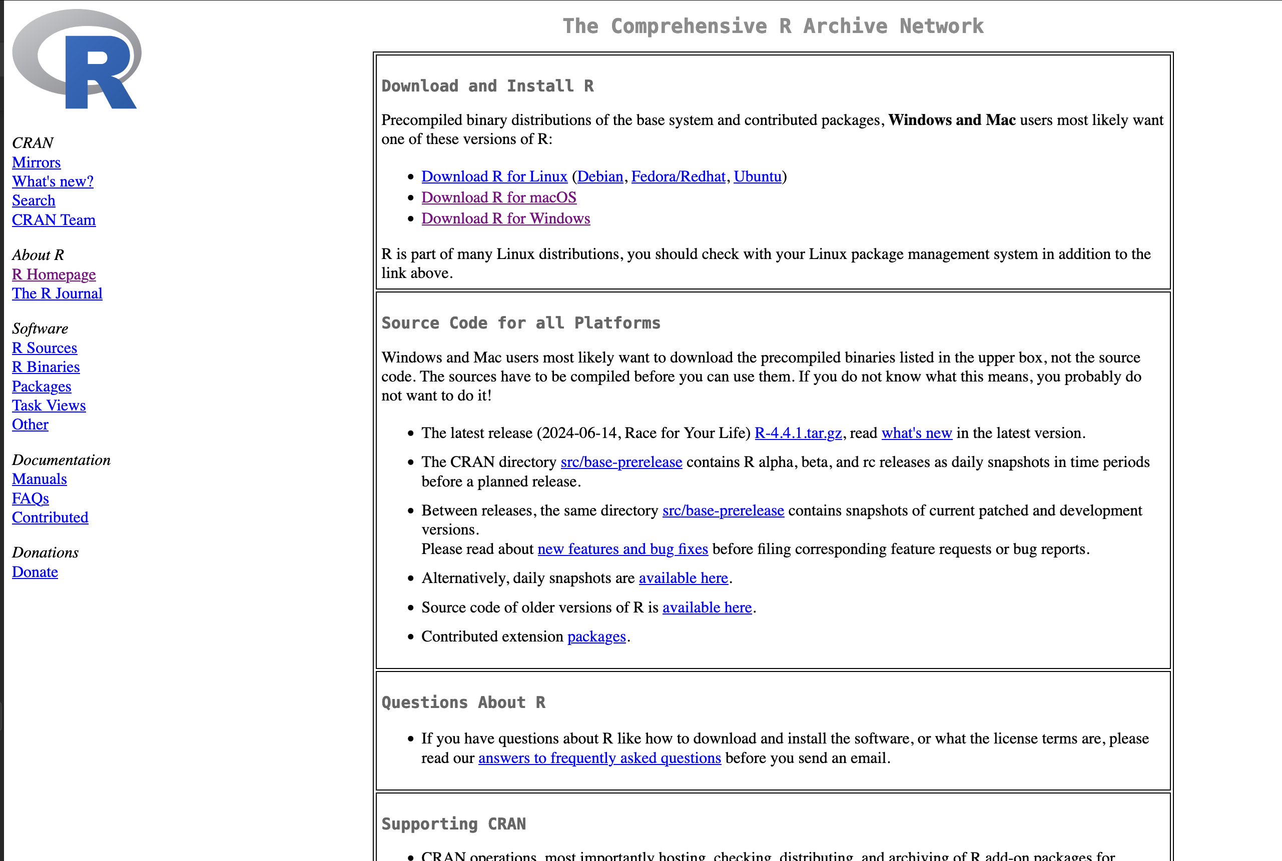
As of 2026-02-18, the most recent version of R is 4.5.2. Using the most current version of R will reduce the likelihood of issues later in the course, so please upgrade even if you already have R installed.
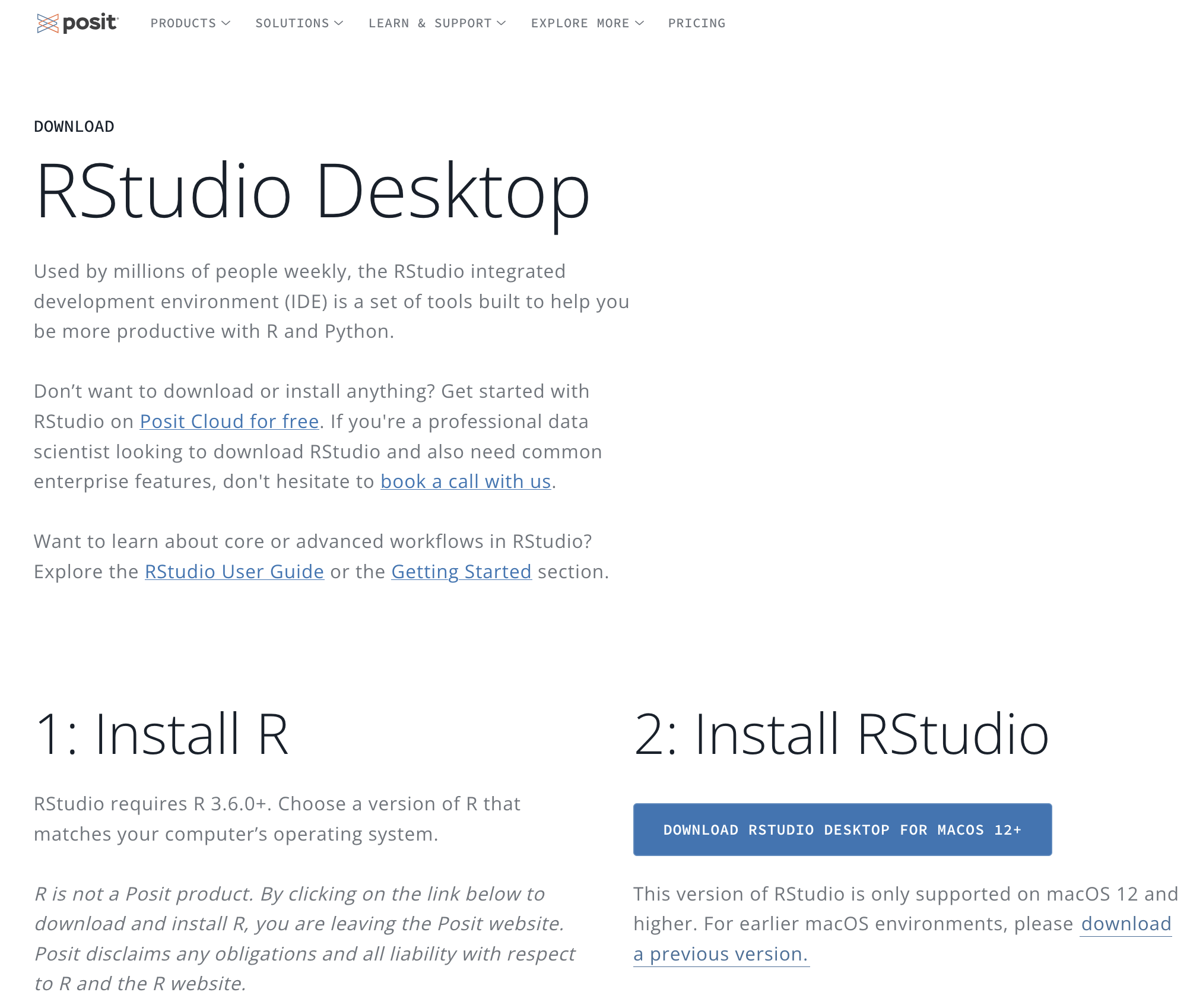
RStudio
Next, download and install the RStudio IDE (desktop edition).
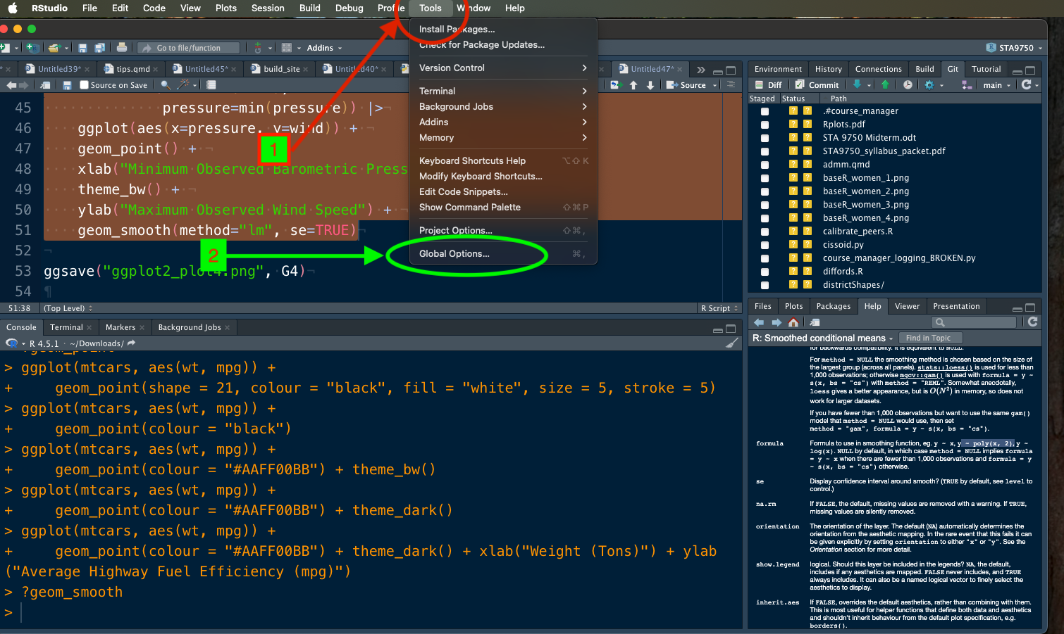
RStudio is highly configurable and I recommend taking advantage of all its built-in features. If you go to the Global Options menu (accessible under Tools1), I recommend the following settings:
- General: Uncheck “Restore .RData into workspace at startup”.
- General: Set “Save workspace to .RData on exit” to “Never”
- Code / Editing: Set “Tab width” to 2
- Code / Editing: Check
- “Insert spaces for Tab”
- Auto-detect code indentation
- Insert matching parens / quotes
- Use native pipe operator
- Auto-indent code after paste
- Vertically align arguments in auto-indent
- Continue comment when inserting new line
- Code / Display: Check
- Show line numbers
- Show margin (margin column should be 80)
- Code / Diagnostics: check all “R” diagnostics.
- Appearance: Pick a color theme you enjoy. (I’m partial to light text on a dark background)
You may wish to enable GitHub Copilot. I have little experience with GH Copilot, but it seems quite popular and is allowed in this course. It is not guaranteed to be accurate at all times - and “the AI told me to” is not a valid excuse if your code is wrong - but on balance, it should be useful.
quarto
We won’t use it this week, but you will need to install Quarto before starting on Mini-Project #00, so if you have a moment, I’d recommend doing it now.
Code Styling
Autoformatting with the styler Package
A major theme of this course will be sharing and co-developing code with your classmates, both for peer feedback and for the course project. Code sharing is hard! Everyone writes code a little differently and what is clear to you may not be clear at all to your reader.
To make code sharing just a bit easier, we use tools to ensure all code shared in this course is consistently formatted. By using consistent formatting, you reduce the cognitive load on your reader, making it easier for them to focus on the ideas of your code, not how you chose to write it.
A major strength of R is its huge number of user-contributed packages. These are “add-ins” which provide additional functionality not available in the basic version of R.
As of 2025-09-25, there are over 22 thousand packages available on CRAN, the largest official repository of R packages. Beyond all those, there are thousands more packages available on other code hosting websites like GitHub.2
We will use the contributed styler package to format code in this course. Run the following command to automatically download and install the styler package:
(Use the clipboard icon on the right of code snippets to automatically copy code suitable for pasting into RStudio.)
You should see something like this:
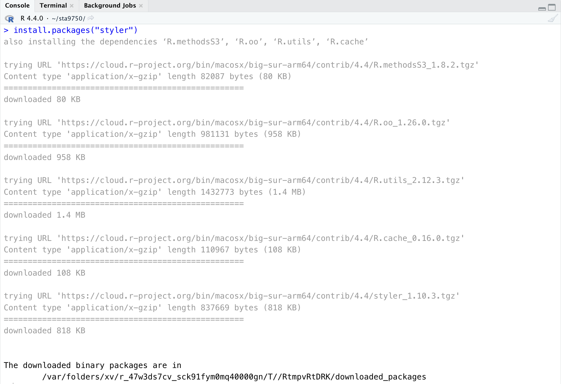
The styler package has been downloaded and installed on your computer, but it is not yet “active” or “open” in R. In general, you will only need to download packages once, but you will need to load them each time you want to use them.3
Open a R file, sometimes called an R script file, in RStudio and copy the following (ugly) code:
if(!require("leaflet")) install.packages("leaflet")
if(!require("tidyverse")){
    install.packages("tidyverse")
   }
 library(tidyverse)
     library(rvest)
library(leaflet)

pAGE = read_html('https://en.wikipedia.org/wiki/Baruch_College')
  pAGE |> html_element(".latitude") |> html_text2() -> BaruchLatitude
  baruch_longitude <- pAGE |> html_element(".longitude") |> html_text2()

    BaruchLatitude <- sum(as.numeric(strsplit(BaruchLatitude,
                                     "[^0123456789]")[[1]]) * (1/60)^(0:2), na.rm=TRUE)
 baruch_longitude <- sum(as.numeric(strsplit(baruch_longitude, "[^0123456789]")[[1]]) *
                             (1/60)^(0:2), na.rm=TRUE)

leaflet() |>
addTiles() |>
    setView(-baruch_longitude, BaruchLatitude,
               zoom=17) |>
    addPopups(-baruch_longitude,
              BaruchLatitude, "Look! It's <b>Baruch College</b>!") |>
print()
You don’t need to understand what this does just yet, but it’s hopefully clear that this is ugly code. Nothing is lined up properly, capitalization is erratic, and different coding styles are intermixed rather recklessly.
Warning
If you run this code and get a Warning message, don’t worry about it for now. Warnings occur when your code runs, but something ‘smelled funny’. At this point, we’re only worrying about an Error message.
Map not Appearing
If the code runs (with Warning) but does not produce a plot, try clicking on the arrow next to the Source button and hitting Source with Echo. This will force R to print the result of the code, i.e., to generate the plot.
Near the top of your RStudio pane, you will see a drop-down menu titled Addins. If you successfully installed styler above, one of the Addins choices will be “style active file.” Click this and the code will be cleaned up (a bit) resulting in something like this:
if (!require("leaflet")) install.packages("leaflet")
if (!require("tidyverse")) {
  install.packages("tidyverse")
}
library(tidyverse)
library(rvest)
library(leaflet)

pAGE <- read_html("https://en.wikipedia.org/wiki/Baruch_College")
pAGE |>
  html_element(".geo") |>
  html_text2() |>
  str_split_1(";") -> BaruchLatitude
baruch_longitude <- pAGE |>
  html_element(".longitude") |>
  html_text2()

BaruchLatitude <- sum(as.numeric(strsplit(
  BaruchLatitude,
  "[^0123456789]"
)[[1]]) * (1 / 60)^(0:2), na.rm = TRUE)
baruch_longitude <- sum(as.numeric(strsplit(baruch_longitude, "[^0123456789]")[[1]]) *
  (1 / 60)^(0:2), na.rm = TRUE)

leaflet() |>
     addTiles() |>
     setView(-baruch_longitude,
             BaruchLatitude,
             zoom = 17) |>
     addPopups(-baruch_longitude,
               BaruchLatitude,
               "Look! It's <b>Baruch College</b>!") |>
     print()
It’s far from perfect - and we will discuss the many issues in this example throughout the course - but it’s better! At a minimum, you should make sure to run styler like this on all code you submit during this course.
And now that your code is cleaned up, you should run it! The Source button in the top right corner will run all code in the open file. Running the code produces something like this:
Not too shabby! That’s an interactive, dynamic map showing the location of Baruch College obtained by parsing the Baruch Wikipedia page, getting the GPS coordinates of Baruch, downloading a map file, and locating Baruch on that map.
Challenge: Adjust this code to show Hunter college instead of Baruch.
More than you ever wanted to know about file types
All the files we use in this course (with very rare exceptions) are some sort of text file in the sense that they are ‘just’ letters in a file. This can be distinguished from file types that contain both text and lots of additional formatting and structure (e.g., a Word document) or are something entirely non-textual (like a picture or a video).
Text files (in this broad sense) are powerful and useful because their simplicity makes them usable and editable by almost anything. You could start writing a file in RStudio, close it and open it in Notepad, make some edits and then close and re-open in another IDE like VSCode, and then final re-open in MS Word without issues. As long as you keep it as a text file – and don’t let Word secretly turn it into a Word document behind your back4 – you maintain full interoperability.
You should distinguish this from something non-plain text like a PDF document. We’ve all had the example of a PDF looking differently on your machine than your friend’s, and not being able to make the edits you want to a PDF unless you pay for a specific piece of expensive software, or having the ability to include videos if you use Adobe Acrobat, but not if you use the PDF viewer built into your browser. This is because a PDF is a complex file format that requires special software to use it and not all software implements everything the exact same way.
A plain text file is sufficiently simple that essentially any software can do anything to it. Because a text file is ‘just’ letters, you can put anything in there:
- R Code
- Python Code
- Simple Notes or SMS (text) messages
- Even something as complex as a plain text spreadsheet. This last one is admittedly a bit obscure and really only appeals to plain-text obsessives.
So then how does software know what to make of a particular plain text file?
This is where file extensions come in: extensions don’t change the contents of a file, they are just a naming convention. But we all agree that if a file is called filename.R, the text in it should be interpreted as R code; a different file called filename.py should be interpreted as python code. You could put R code in a .py file and it would still be a file, but when you then started up Python instead of R, you’d get all sorts of errors.5
File extensions naming conventions are purely social conventions. But social conventions are powerful!
When you ask R studio to open a .R file, it assumes you’re going to do “R things” with it. And so it gives you buttons to “Run” or “Source” the code by default; those buttons are hooked up to the R interpreter, the actual software that does ‘R things’. These buttons aren’t inherent to the file or hidden in its contents anywhere: the buttons are only added by RStudio as it tries to be as helpful as possible.
If you instead ask RStudio to open a .py file, it will presnet you some python-related buttons by default. And if you ask RStudio to open a .qmd file, it will give you buttons to “Render” default.
So any plain text file can theoretically be anything. It’s just the file extension gives RStudio a hint as to what to you’re going to do with and RStudio uses that hint to (try to) be helpful to you. At the time of file creation (i.e., the New File menu), RStudio can’t get this social clue from the file name since it’s never been saved and no filename exists, so it asks you directly.
If you open a file in RStudio and want it to be treated differently, you can click the little text in the bottom right of the file. If you start with an .R file (or the “R Script” new file menu), this will say R Script. If you instead change that to something like “Quarto”, you’ll see the buttons at the top change to the Quarto related buttons. In doing this, you’re not actually changing the file, you’re just telling RStudio to give you different tools for working with that file.
So what does this mean for you in this class?
- Everything we’ll do in this class is some sort of ‘plain text file’
- All plain text files are internally the same - we just add social conventions around them based on their names and extensions (
test.Rvstest.qmdvstest.txt) - RStudio knows these social conventions and tries to play along, but can be overruled.
So, the right file type reflects what you want to do:
if you’re using this code for just plain R code and nothing else, you want
RStudioto interpret it as anR Scriptand you should proceed accordingly, by naming itfilename.Rand by using the “R Script” type when creating a new file. If you’re saving a new file of this type, RStudio will encourage (but not insist) you save it as.Rto convey your intention to your future self and RStudio when it re-opens the file later.If you want to write a Quarto document and have the ability to mix in code and text, with the goal of producing a ‘document’ output (e.g., a web page or a PDF), you should make sure your file is named
filename.qmd(if it already exists) or create it by using the “Quarto Document” type in the new file menu.If you want to write a document that is just text to be read by a human and no other purpose (e.g., a personal TODO list or a draft of an email before you copy it into Outlook), the social convention is that this is either a
.txtfile or a file with no extension at all (likeREADME). Somewhat confusingly, this particular social convention is also called a “text file” in the narrow sense of being English language text, as distinct from the “text file” in the sense of being letters and not binary code or photos I’ve been using up to this point. The RStudio new file menu will call this a “Text File” and will default to saving it as a.txtfile.
lintr
If you want even more feedback on writing good code, install the lintr package and use the associated RStudio add-in. Unlike styler, lintr won’t make changes automatically for you, but it will highlight much more subtle possible problems.6
Source Code Management
git
git is a source-code management tool, used by developers to manage the code they write. If you’ve ever been part of a large project and struggled to coordinate all team members using the same version of a document, git exists to solve that problem.
If you don’t have git pre-installed, install either Git for Windows or the XCode Command Line Tools for MacOS7 as appropriate.
In this course, we will use three main functions of git:
-
staging: telling
git, I want you to prepare to save a certain file - committing: saving a set of related changes
- pushing: copying your committed changes to a separate server for sharing and backup
Whenever you write code you are happy with, you should use git to save it. Saving changes with git is cheap and easy - so do it regularly. You always want git to have a backup of good code in case you loose power, accidentally delete a file, break something in a way you’re not sure how to undo, etc..
RStudio comes with powerful git integration. Once you have created a project, you should see a tab labelled “Git” in the top right corner of your IDE window that looks something like this:
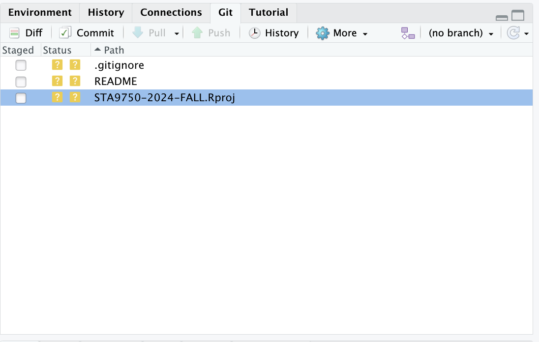
For this semester, you should create a project called STA9750-2026-SPRING. It is very important that you copy this name exactly and maintain both the hyphens and the capitalization. All work for this course will live within this project. We will discuss the use of projects in more detail in Mini-Project #00.
To stage a file - prepare to save it - click the empty check box next to the file name. A new file shows a status of “?” - this is git saying “I’ve never seen this file before. Do you want me to track it for you?”. Later, when you make further changes to file you have already asked git to track, a status of “M” (for Modified) will be shown.
On its own staging a file does nothing. You also need to commit it for git to truly track it.8 The Commit button will commit all staged changes. When you make a commit, git requires a brief message summarizing the changes. There’s no particular formatting requirement to this message, but it should be something that future-you is able to easily understand. For instance, the commit message from the initial draft of this document reads as:
Initial draft of Lab 01 (STA9750)

- Installing R and RStudio
- Git and GitHub
- Leaflet Example for Styler

TODO: Fuller shell explainers
TODO: Link more git help
When I read this, I know the purpose of the change I made (first line), the contents of that change (list), and parts that still need more work.
Finally, after you save a change, it is only saved on your computer. The true power of git comes from its ability to copy changes and backups across machines. This gives you an easy way to store backups in case your computer dies and makes collaboration efficient and fun. git allows you to push and pull changes between machines in endlessly powerful (but sometimes complex) ways. For this course, we’ll keep things simple and only use GitHub to share code. We discuss GitHub in the next section.
Reference: We will not use all of the functionality of git in this course, but you should familiarize yourself with Chapters 1, 2, and 6 of the Git Book over the next two weeks.
GitHub
GitHub is an industry-standard code hosting and collaboration platform. In addition to hosting copies of code, GitHub provides web hosting, bug reporting, code review, continuous integration, documentation wikis, and discussion fora. You will explore GitHub in more detail starting in Mini-Project #00.
Extra: Welcome to $SHELL
To become a true “power user” of tools like R and python, you will need to become more familiar with the command line interface (CLI) and associated tools.9
The Software Carpentry Unix Shell Tutorial is a great introduction to shell usage. Check it out!
NB: MacOS and Linux systems work quite similarly under the hood, as both descend from the Unix tradition. By contrast, Windows works somewhat differently. Learners whose personal machine runs Windows are encouraged to take advantage of the provided Linux-running virtual machines10 as they work through this section.
Looking Ahead
Next week, we will use these tools to begin coding in earnest. If you’re feeling ambitious, go ahead and get started on Mini-Project #00.
Footnotes
-
On a Mac, the
Global Options >> Toolsmenu is available at the same place you’ll find options for almost all Mac software: along the very top bar of the screen when you are in the relevant app. If you don’t see this bar, you need to exit full screen mode. Note that this is a Mac-wide way of displaying and hiding menus, and is not specific toRStudio. On a Windows machine, the tools are usually located near the top of the RStudio window, not near the top of the entire display. If you are interested in bioinformatics, the Bioconductor project develops incredible open-source
Rpackages.↩︎While this may feel cumbersome, it’s really not dissimilar to any other software you use (or
Ritself). You need to download it once, but you need to open it each time you intend to use it. There’s no harm in re-downloading–free software!–but it wastes time and bandwidth. Since we benefit so much from the free-software community, the very least we can do is not run up their internet bills unnecessarily.↩︎If you open a non-
docxfile in Word and edit it, Word will give you a scary warning message about ‘loosing features’ if you don’t convert to a MS Word format. That message is more of a scare tactic to get you to only use Word and avoid other software than anything you should actually credit.↩︎-
It is theoretically possible to have a bit of code that is so simple, it is both valid
Rcode andpythoncode. In that case, you could try to run that file inRand inpythonand everything would be ok. As far as theRsoftware or thepythonsoftware care, it’s just text. It only becomes code when theRsoftware or thepythonsoftware try to use it as code.For example, a file that contains only these lines
print(hello)could be run with
Rto produce the output:% Rscript test.txt [1] "Hello!"If we instead run the same file with the
pythoncommand, we would get similar (but not quite identical) output:% python test.txt Hello!But this is a sort of trivial example that doesn’t extend to software that does anything actually interesting.↩︎
Some of the issues identified by
lintrmay be false positives, but the false positive rate is quite low, especially for the sort of procedural code that is the focus of this course. You should default to trying to appeaselintr, but feel free to use the course discussion board for any questions.↩︎-
XCode is a bundle of useful software development tools that Apple makes available for anyone using a Mac. One of those tools is
git, so this makes XCode the “most official” way to installgiton a Mac. If you click on the “Terminal” tab in RStudio (just to the right of “Console” in the bottom left quadrant) and type:gitNote that this must be run at a Mac command line, not at the
Rconsole. The command line is direct control of the operating system itself, while theRconsole is just for controllingR. WithinRStudio, you can access the command line by clicking on theTerminaltab, located near theConsoletab.After running
git, you will be able to determine ifgitis already installed. Ifgitis installed, you will receive either a long-ish help message telling you how to usegitor a status message for your currentgitrepository. Either of these means you already havegitinstalled.If
gitis not installed, recent-ish Macs usually will offer to installgitfor you when you try to run it. A pop-up window will appear and ask if you want to install XCode. XCode contains many tools and is a bit large, so this installation may take over an hour. If, for whatever reason, the pop up menu does not appear, simply runxcode-select --installat the
Terminaland it will install XCode (includinggit) for you. You may need to type your computer password here. If you are working in a terminal and no letters appear when start to type your password, don’t worry: that is just a standard security precaution.↩︎ This two stage process is a bit cumbersome for the first stage of a small project, but it quickly becomes incredibly valuable. Instead of saving everything every time, there is great power in only saving “good” or “finished” changes to a large project, while leaving work-in-progress elsewhere unsaved. You probably won’t need this level of control until you get to the course project, but it’s better to have it than not.↩︎
As an added benefit, use of the CLI also makes you look like a 90s movie hacker to all your friends.↩︎
See the Course Resources page.↩︎