STA 9750 Week 4 Pre Assignment: Single-Table dplyr Verbs

Due Date: 2024-09-18 (Wednesday) at 11:45pm

Submission: CUNY Brightspace

This week, we begin manipulating R’s most important structure the data.frame. While base R provides tools for working with data.frame objects, our primary focus will be on the tidyverse family of tools. These provide a unified and consistent set of tools for working with data objects.

What is a data.frame?

Last week, we discussed vectors, one-dimensional collections of the same type of object. While vectors are an important computational tool, real data is rarely quite so simple: we collect multiple features (covariates) from each of our observations and these features may be of different type. For example, when performing a political survey, we may record the:

• Name (character)
• Age (integer)
• Gender (factor)¹
• Date of Contact (Date)
• Level of candidate support (double or numeric)

of each respondant. It is natural to organize this in tabular (“spreadsheet”) form:

Name	Age	Gender	Date of Contact	Level of Support
Timmy	25	M	2024-09-13	0.25
Tammy	50	F	2024-06-20	-1.35
Taylor	70	X	2024-08-15	200
Tony	40	M	2024-12-25	0
Toni	65	F	2024-11-28	-4

Note several important features of this data:

• Each row corresponds to one, and only one, sample
• Each column corresponds to one, and only one, feature
• The values in each column are all of the same type
• The order doesn’t matter: all important data is reflected in the values, not the presentation

Generally, data in this pattern will be called “tidy”. R represents this type of data as a data.frame object. For more on what it means for data to be “tidy”, read this paper.

Tibbles and the Tidyverse

Many of the tools we will discuss in this class are from a set of related R packages, collectively known as the tidyverse. They are designed to i) read data from outside of R into tidy formats; ii) manipulate data from one tidy format to another; iii) communicate the results of tidy data analyses.

While you can load these packages separately, they are used together so frequently that the tidyverse package exists to load them all simultaneously. I recommend you start most of your analyses with the command:

library(tidyverse)

This will automatically load the following packages:

• lubridate for date and time manipulation
• forcats for factor manipulation
• stringr for string manipulation
• dplyr for data frame manipulation
• purrr for functional programming
• readr for tidy data import
• tidyr for tidy data manipulation
• tibble for data frame enhancement
• ggplot2 for data visualization

This week, we are focusing on functionality from the dplyr package.

You may, from time to time, see reference to tibbles in R documentation. A tibble is a “souped-up” data frame with somewhat better default printing. For almost all purposes-and everywhere in this course- you can substitute tibble with data.frame without issue.

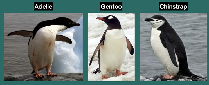
Before we get into dplyr, let’s make sure we have a data frame to play with. Let’s bring back our friends, the Palmer penguins:

library(tidyverse)
library(palmerpenguins)
penguins

# A tibble: 344 × 8
   species island    bill_length_mm bill_depth_mm flipper_length_mm body_mass_g
   <fct>   <fct>              <dbl>         <dbl>             <int>       <int>
 1 Adelie  Torgersen           39.1          18.7               181        3750
 2 Adelie  Torgersen           39.5          17.4               186        3800
 3 Adelie  Torgersen           40.3          18                 195        3250
 4 Adelie  Torgersen           NA            NA                  NA          NA
 5 Adelie  Torgersen           36.7          19.3               193        3450
 6 Adelie  Torgersen           39.3          20.6               190        3650
 7 Adelie  Torgersen           38.9          17.8               181        3625
 8 Adelie  Torgersen           39.2          19.6               195        4675
 9 Adelie  Torgersen           34.1          18.1               193        3475
10 Adelie  Torgersen           42            20.2               190        4250
# ℹ 334 more rows
# ℹ 2 more variables: sex <fct>, year <int>

Subsetting Data Frames

Our first task will be to subset data frames: that is, to select only some rows and columns and to return a smaller data frame than the one we started with.

Subsetting Columns

The main dplyr function for column subsetting is select(). In its simplest form, we provide a set of column names we want to keep and everything else gets dropped.

select(penguins, species, island)

# A tibble: 344 × 2
   species island   
   <fct>   <fct>    
 1 Adelie  Torgersen
 2 Adelie  Torgersen
 3 Adelie  Torgersen
 4 Adelie  Torgersen
 5 Adelie  Torgersen
 6 Adelie  Torgersen
 7 Adelie  Torgersen
 8 Adelie  Torgersen
 9 Adelie  Torgersen
10 Adelie  Torgersen
# ℹ 334 more rows

Here, we keep the species and island columns and remove the others.

Pause for a moment to note how the select function is structured: the first argument is the data frame on which we are operating; all following arguments control the resulting behavior. This is a common pattern in dplyr functions, designed to take advantage of another key R functionality, the pipe operator.

R provides an operator |> which “rewrites” code, so

select(penguins, species, island)

and

penguins |> select(species, island)

are exactly the same thing as far as R is concerned. You may well ask yourself why bother: the second “piped” operator is a bit longer and a bit harder to type. But just hold on - we’ll see this makes for far cleaner code in the long run.

Just like base R, if we include - signs in our select statement, we get everything except a certain column:

penguins |> select(-bill_length_mm, -bill_depth_mm, -flipper_length_mm)

# A tibble: 344 × 5
   species island    body_mass_g sex     year
   <fct>   <fct>           <int> <fct>  <int>
 1 Adelie  Torgersen        3750 male    2007
 2 Adelie  Torgersen        3800 female  2007
 3 Adelie  Torgersen        3250 female  2007
 4 Adelie  Torgersen          NA <NA>    2007
 5 Adelie  Torgersen        3450 female  2007
 6 Adelie  Torgersen        3650 male    2007
 7 Adelie  Torgersen        3625 female  2007
 8 Adelie  Torgersen        4675 male    2007
 9 Adelie  Torgersen        3475 <NA>    2007
10 Adelie  Torgersen        4250 <NA>    2007
# ℹ 334 more rows

Here, we dropped three columns.

The select operator provides more advanced functionality which is useful for very complex data structures, but we don’t need to dive into that just yet.

Subsetting Rows

Often in data analysis, we want to focus on a subset of the entire population: e.g., we might want to know the fraction of women supporting a certain political candidate or the rate of a rare cancer among patients 65 or older. In this case, we need to select only those rows of our data that match some criterion. This brings us to the filter operator.

filter takes a logical vector and uses it to select rows of a data frame. Most commonly, this logical vector is created by performing some sort of tests on the values in the data frame. For example, if we want to select only the male penguins in our data set, we may write:

penguins |> filter(sex == "male")

# A tibble: 168 × 8
   species island    bill_length_mm bill_depth_mm flipper_length_mm body_mass_g
   <fct>   <fct>              <dbl>         <dbl>             <int>       <int>
 1 Adelie  Torgersen           39.1          18.7               181        3750
 2 Adelie  Torgersen           39.3          20.6               190        3650
 3 Adelie  Torgersen           39.2          19.6               195        4675
 4 Adelie  Torgersen           38.6          21.2               191        3800
 5 Adelie  Torgersen           34.6          21.1               198        4400
 6 Adelie  Torgersen           42.5          20.7               197        4500
 7 Adelie  Torgersen           46            21.5               194        4200
 8 Adelie  Biscoe              37.7          18.7               180        3600
 9 Adelie  Biscoe              38.2          18.1               185        3950
10 Adelie  Biscoe              38.8          17.2               180        3800
# ℹ 158 more rows
# ℹ 2 more variables: sex <fct>, year <int>

Here, note the use of the == operator for testing equality. A very common mistake is to use the single equals (assignment) operator inside of filter. Thankfully, dplyr will alert us with an error if we make this mistake:

penguins |> filter(sex = "male")

Error in `filter()`:
! We detected a named input.
ℹ This usually means that you've used `=` instead of `==`.
ℹ Did you mean `sex == "male"`?

If we supply multiple tests to filter, we get the intersection: that is, we get rows that pass all tests.

penguins |> filter(sex == "male", bill_length_mm > 38)

# A tibble: 156 × 8
   species island    bill_length_mm bill_depth_mm flipper_length_mm body_mass_g
   <fct>   <fct>              <dbl>         <dbl>             <int>       <int>
 1 Adelie  Torgersen           39.1          18.7               181        3750
 2 Adelie  Torgersen           39.3          20.6               190        3650
 3 Adelie  Torgersen           39.2          19.6               195        4675
 4 Adelie  Torgersen           38.6          21.2               191        3800
 5 Adelie  Torgersen           42.5          20.7               197        4500
 6 Adelie  Torgersen           46            21.5               194        4200
 7 Adelie  Biscoe              38.2          18.1               185        3950
 8 Adelie  Biscoe              38.8          17.2               180        3800
 9 Adelie  Biscoe              40.6          18.6               183        3550
10 Adelie  Biscoe              40.5          18.9               180        3950
# ℹ 146 more rows
# ℹ 2 more variables: sex <fct>, year <int>

If we want the union-rows that satisfy any of the tests-we have to use the logical operators we previous applied to vectors:

penguins |> filter( (sex == "male") | (bill_length_mm > 38))

# A tibble: 292 × 8
   species island    bill_length_mm bill_depth_mm flipper_length_mm body_mass_g
   <fct>   <fct>              <dbl>         <dbl>             <int>       <int>
 1 Adelie  Torgersen           39.1          18.7               181        3750
 2 Adelie  Torgersen           39.5          17.4               186        3800
 3 Adelie  Torgersen           40.3          18                 195        3250
 4 Adelie  Torgersen           39.3          20.6               190        3650
 5 Adelie  Torgersen           38.9          17.8               181        3625
 6 Adelie  Torgersen           39.2          19.6               195        4675
 7 Adelie  Torgersen           42            20.2               190        4250
 8 Adelie  Torgersen           41.1          17.6               182        3200
 9 Adelie  Torgersen           38.6          21.2               191        3800
10 Adelie  Torgersen           34.6          21.1               198        4400
# ℹ 282 more rows
# ℹ 2 more variables: sex <fct>, year <int>

It’s a bit clunky, but thankfully, this is somewhat less common than checking that all conditions are satisfied.

dplyr provides all sorts of useful helpers for creating test statements, e.g., the

• between
• near

functions.

Even more useful than these, however, are the slice_*() functions which can be used to perform “top \(k\)” type operations. If we want the five largest Adelie penguins, we might try something like:

penguins |> filter(species == "Adelie") |> slice_max(body_mass_g, n=5)

# A tibble: 5 × 8
  species island    bill_length_mm bill_depth_mm flipper_length_mm body_mass_g
  <fct>   <fct>              <dbl>         <dbl>             <int>       <int>
1 Adelie  Biscoe              43.2          19                 197        4775
2 Adelie  Biscoe              41            20                 203        4725
3 Adelie  Torgersen           42.9          17.6               196        4700
4 Adelie  Torgersen           39.2          19.6               195        4675
5 Adelie  Dream               39.8          19.1               184        4650
# ℹ 2 more variables: sex <fct>, year <int>

slice_min() works similarly. slice_head and slice_tail get the first and last rows by sort order - in general, I recommend against using these. A key rule of data analysis is that the row order is not semantically meaningful, but it’s good to keep them in the back of your mind just in case. slice_sample can be used to select random subsets of data.

Another important subseting function is drop_na which will drop any rows with missing (NA) data.² This is a good and useful tool, but before you apply it, always ask yourself “why is this data missing?” Understanding the abscence of data is often just as important as understanding the non-missing data. For example, is a student’s SAT score missing on a college application because they i) forgot to list it; ii) never took the SAT; or iii) took the test but chose to omit their score because they did poorly? Proper handling of missing data is often very problem-specific and very hard.

Manipulating and Creating Columns

A key task in data analysis is transforming data. As discussed in class, one of the guiding themes of R programming is data integrity and an important way R ensures this is by applying commands to the entire vector. In the data frame context, we apply commands to an entire column. The mutate function is dplyr’s main interface for column creation and manipulation.

In general, each argument to mutate takes a name = value pair: the name is the name of a column to be created from value. value can be an arbitrary function of other columns. If name corresponds to an existing column, that column is silently overwritten.

For example, if we want to convert penguin bill lengths from millimeters to inches, we might operator:

penguins |> mutate(bill_length_in = bill_length_mm / 25.4)

# A tibble: 344 × 9
   species island    bill_length_mm bill_depth_mm flipper_length_mm body_mass_g
   <fct>   <fct>              <dbl>         <dbl>             <int>       <int>
 1 Adelie  Torgersen           39.1          18.7               181        3750
 2 Adelie  Torgersen           39.5          17.4               186        3800
 3 Adelie  Torgersen           40.3          18                 195        3250
 4 Adelie  Torgersen           NA            NA                  NA          NA
 5 Adelie  Torgersen           36.7          19.3               193        3450
 6 Adelie  Torgersen           39.3          20.6               190        3650
 7 Adelie  Torgersen           38.9          17.8               181        3625
 8 Adelie  Torgersen           39.2          19.6               195        4675
 9 Adelie  Torgersen           34.1          18.1               193        3475
10 Adelie  Torgersen           42            20.2               190        4250
# ℹ 334 more rows
# ℹ 3 more variables: sex <fct>, year <int>, bill_length_in <dbl>

Here, note that the bill_length_mm column is retained - and all columns are kept! mutate only creates new columns; it won’t secretly drop them.

A particularly common operator is changing the name of a column without changing its values. You can use mutate and select(-) for this, but rename provides essentially the same interface and its semantically clearer:

penguins |> rename(mass = body_mass_g)

# A tibble: 344 × 8
   species island    bill_length_mm bill_depth_mm flipper_length_mm  mass sex   
   <fct>   <fct>              <dbl>         <dbl>             <int> <int> <fct> 
 1 Adelie  Torgersen           39.1          18.7               181  3750 male  
 2 Adelie  Torgersen           39.5          17.4               186  3800 female
 3 Adelie  Torgersen           40.3          18                 195  3250 female
 4 Adelie  Torgersen           NA            NA                  NA    NA <NA>  
 5 Adelie  Torgersen           36.7          19.3               193  3450 female
 6 Adelie  Torgersen           39.3          20.6               190  3650 male  
 7 Adelie  Torgersen           38.9          17.8               181  3625 female
 8 Adelie  Torgersen           39.2          19.6               195  4675 male  
 9 Adelie  Torgersen           34.1          18.1               193  3475 <NA>  
10 Adelie  Torgersen           42            20.2               190  4250 <NA>  
# ℹ 334 more rows
# ℹ 1 more variable: year <int>

Operating with Group Structure

We often want to summarize our data in useful ways: these can be simple summaries like mean (average) or standard deviation or more complex operations (trend lines). In the world of dplyr, the summarize function is used whenever we want to reduce multiple rows to a single data point. Note how this differs from filter: filter drops rows, summarize combines and reduces them.

For example, if we want to get the number of male penguins in our data set, we can use the n() function, which counts the number of rows:

penguins |> summarize(number = n())

# A tibble: 1 × 1
  number
   <int>
1    344

Look at all those penguins!

This is a relatively simple operation, but we can be a bit more complex: e.g., with the mean function:

penguins |> summarize(body_mass_avg = mean(body_mass_g))

# A tibble: 1 × 1
  body_mass_avg
          <dbl>
1            NA

Wait! Why didn’t that work?

Recall that the penguins data had some missing (NA) values. When we ask R to compute the average, it can’t! Specifically, depending on the missing values, the mean could be anything, so R returns a missing (unknown) value for the mean as well. Many base R functions have this default behavior and have an optional flag for automatically removing NA values:

penguins |> summarize(body_mass_avg = mean(body_mass_g, na.rm=TRUE))

# A tibble: 1 × 1
  body_mass_avg
          <dbl>
1         4202.

Here na.rm=TRUE means to remove all na values before computing the mean.

The summarize function is particularly powerful when applied groupwise: e.g., what is the average body mass by species? In dplyr world, this is a two-step operation:

penguins |> 
    group_by(species) |>
    summarize(body_mass_avg = mean(body_mass_g, na.rm=TRUE))

# A tibble: 3 × 2
  species   body_mass_avg
  <fct>             <dbl>
1 Adelie            3701.
2 Chinstrap         3733.
3 Gentoo            5076.

We added the group_by operator here. Note that, on its own, group_by doesn’t really do anything:

penguins |> 
    group_by(species)

# A tibble: 344 × 8
# Groups:   species [3]
   species island    bill_length_mm bill_depth_mm flipper_length_mm body_mass_g
   <fct>   <fct>              <dbl>         <dbl>             <int>       <int>
 1 Adelie  Torgersen           39.1          18.7               181        3750
 2 Adelie  Torgersen           39.5          17.4               186        3800
 3 Adelie  Torgersen           40.3          18                 195        3250
 4 Adelie  Torgersen           NA            NA                  NA          NA
 5 Adelie  Torgersen           36.7          19.3               193        3450
 6 Adelie  Torgersen           39.3          20.6               190        3650
 7 Adelie  Torgersen           38.9          17.8               181        3625
 8 Adelie  Torgersen           39.2          19.6               195        4675
 9 Adelie  Torgersen           34.1          18.1               193        3475
10 Adelie  Torgersen           42            20.2               190        4250
# ℹ 334 more rows
# ℹ 2 more variables: sex <fct>, year <int>

We have added some grouping metadata but the actual data does not get changed until the summarize step.

We can also group by more than one element:

penguins |> 
    group_by(species, sex) |>
    summarize(body_mass_avg = mean(body_mass_g, na.rm=TRUE))

`summarise()` has grouped output by 'species'. You can override using the
`.groups` argument.

# A tibble: 8 × 3
# Groups:   species [3]
  species   sex    body_mass_avg
  <fct>     <fct>          <dbl>
1 Adelie    female         3369.
2 Adelie    male           4043.
3 Adelie    <NA>           3540 
4 Chinstrap female         3527.
5 Chinstrap male           3939.
6 Gentoo    female         4680.
7 Gentoo    male           5485.
8 Gentoo    <NA>           4588.

Note here that the result is still grouped and that only the last (sex) grouping was removed. That means that any future operations will be automatically grouped by species. If you want to remove all grouping structure, add the ungroup operator at the end:

penguins |> 
    group_by(species, sex) |>
    summarize(body_mass_avg = mean(body_mass_g, na.rm=TRUE)) |>
    ungroup()

`summarise()` has grouped output by 'species'. You can override using the
`.groups` argument.

# A tibble: 8 × 3
  species   sex    body_mass_avg
  <fct>     <fct>          <dbl>
1 Adelie    female         3369.
2 Adelie    male           4043.
3 Adelie    <NA>           3540 
4 Chinstrap female         3527.
5 Chinstrap male           3939.
6 Gentoo    female         4680.
7 Gentoo    male           5485.
8 Gentoo    <NA>           4588.

group_by metadata is also useful when summary statistics are computed implicitly by other functions. E.g., if we want to get all penguins that are above average mass for their species, we might try the following:

penguins |> 
    group_by(species) |>
    filter(body_mass_g >= mean(body_mass_g, na.rm=TRUE)) |>
    ungroup()

# A tibble: 159 × 8
   species island    bill_length_mm bill_depth_mm flipper_length_mm body_mass_g
   <fct>   <fct>              <dbl>         <dbl>             <int>       <int>
 1 Adelie  Torgersen           39.1          18.7               181        3750
 2 Adelie  Torgersen           39.5          17.4               186        3800
 3 Adelie  Torgersen           39.2          19.6               195        4675
 4 Adelie  Torgersen           42            20.2               190        4250
 5 Adelie  Torgersen           38.6          21.2               191        3800
 6 Adelie  Torgersen           34.6          21.1               198        4400
 7 Adelie  Torgersen           42.5          20.7               197        4500
 8 Adelie  Torgersen           46            21.5               194        4200
 9 Adelie  Biscoe              35.9          19.2               189        3800
10 Adelie  Biscoe              38.2          18.1               185        3950
# ℹ 149 more rows
# ℹ 2 more variables: sex <fct>, year <int>

Here, R applies the summarization function mean groupwise for us.

Before we close out, let’s put this all together: what species has the largest difference in average body mass between the sexes?

Answer: Gentoo penguins have the largest sex difference in average body mass.

Before completing the Brightspace submission for this assignment, look up the source for this document on my GitHub (Hint: see the buttons on the sidebar) and see i) how I computed the answer; and ii) how I included it in the rendered text. This will be helpful as you begin preparing your first report.

Footnotes

1. Recall a factor is a vector with a fixed set of possible values, often used to represent categorical data. Here, we follow the NY DMV and allow M, F, and X values for sex, but, in general, representation of sex and gender in databases is a tricky problem. See this essay for a list of some of the complexity of real people. (This essay follows in a longer tradition of “the world is much more complicated than you would believe” essays: names, time, addresses. People - and the world we create - are infinitely complex.

2. We will say much more about R’s missing data model in a few weeks.