| Date | Time | Details |
|---|---|---|
| 2026-03-12 | 6:00pm ET | Pre-Assignment #06 Due |
| 2026-03-13 | 11:59pm ET | Mini-Project #01 Due |
| 2026-03-19 | 6:00pm ET | Pre-Assignment #07 Due |
| 2026-03-22 | 11:59pm ET | Mini-Project Peer Feedback #01 Due |
| 2026-03-26 | 6:00pm ET | Mid-Semester Check-In Slides Due |
| 2026-04-02 | 11:59pm ET | Mid-Semester Teammate Peer Evaluations Due |
| 2026-04-02 | NA | Classes Cancelled (Spring Break – Week 1) |
Software Tools for Data Analysis
STA 9750
Michael Weylandt
Week 5 – Thursday 2026-03-05
Last Updated: 2026-03-05
STA 9750 Week 5
Today: Lecture #04: Single Table dplyr Verbs
These slides can be found online at:
In-class activities (if any) can be found at:
Upcoming TODO
Upcoming student responsibilities:
STA 9750 Week 5
Today: Lecture #04: Single Table dplyr Verbs
Mini-Project #01
Mini-Project #01 due on 2026-03-13 at 11:59pm ET:
Assessing the Impact of SFFA on Campus Diversity One-Year Later
Topics Covered:
- Reproducible Research Tooling
- Packages and Functions
- Basic Data Manipulation (Today)
- Tables for Data Display (In Assignment)
Not everything has a single right answer - be reasonable, justify, and document
MP#01 Analysis
Analysis:
- College Enrollment
- Steps:
- Data Import and Preparation
- Initial Exploration
- Writing Op-Ed
- Practice
dplyrsingle-table calculations
MP#01 Formatting
Formatting:
qmddocument- “Op-Ed” + supporting analysis
- Put Op-Ed at beginning or end, clearly identified
Submission:
- Push to
GitHub - Tag on GitHub issues (
mp_submission_create) - Print to PDF + Submit on Brightspace
MP#01 Rubric
- 8 graded sections (out of 10)
- 3 automatic 10 as long as you copy+paste my code and follow my EDA
Today
Today
- Brief Review
- Single-Table Verbs
- Introduction to MP#01
- Pre-Assignment #04 FAQs
- Wrap-Up
Brief Review
Vectors
A vector is R’s basic data type:
- Fixed length, ordered, same class
Vectors
By default, R tries to respect vector structure in calculations:
Packages
Packages provide additional functionality:
install.packagesone time to download from CRAN (online repository)libraryeach time to activate package before use
No ‘cost’ to running library repeatedly - include as needed if uncertain
Not Found Errors
Common error:
Three checks:
- Spelling errors
- Do you need to load a package?
- Did you run code to define variable above?
Particularly common when moving code into quarto since quarto runs everything “fresh”: all of the code in the qmd and only the code in the qmd
Single-Table Verbs
data.frame
Last week: Vectors
- 1D structures of same type
- Vectorized semantics
- Building blocks of more complex structures
Today: data.frames
data.frame
penguins is a data frame included in recent versions of R
species island bill_len bill_dep flipper_len body_mass sex year
1 Adelie Torgersen 39.1 18.7 181 3750 male 2007
2 Adelie Torgersen 39.5 17.4 186 3800 female 2007
3 Adelie Torgersen 40.3 18.0 195 3250 female 2007
4 Adelie Torgersen NA NA NA NA <NA> 2007
5 Adelie Torgersen 36.7 19.3 193 3450 female 2007
6 Adelie Torgersen 39.3 20.6 190 3650 male 2007
7 Adelie Torgersen 38.9 17.8 181 3625 female 2007
8 Adelie Torgersen 39.2 19.6 195 4675 male 2007
9 Adelie Torgersen 34.1 18.1 193 3475 <NA> 2007
10 Adelie Torgersen 42.0 20.2 190 4250 <NA> 2007
11 Adelie Torgersen 37.8 17.1 186 3300 <NA> 2007
12 Adelie Torgersen 37.8 17.3 180 3700 <NA> 2007
13 Adelie Torgersen 41.1 17.6 182 3200 female 2007
14 Adelie Torgersen 38.6 21.2 191 3800 male 2007
15 Adelie Torgersen 34.6 21.1 198 4400 male 2007
16 Adelie Torgersen 36.6 17.8 185 3700 female 2007
17 Adelie Torgersen 38.7 19.0 195 3450 female 2007
18 Adelie Torgersen 42.5 20.7 197 4500 male 2007
19 Adelie Torgersen 34.4 18.4 184 3325 female 2007
20 Adelie Torgersen 46.0 21.5 194 4200 male 2007
21 Adelie Biscoe 37.8 18.3 174 3400 female 2007
22 Adelie Biscoe 37.7 18.7 180 3600 male 2007
23 Adelie Biscoe 35.9 19.2 189 3800 female 2007
24 Adelie Biscoe 38.2 18.1 185 3950 male 2007
25 Adelie Biscoe 38.8 17.2 180 3800 male 2007
26 Adelie Biscoe 35.3 18.9 187 3800 female 2007
27 Adelie Biscoe 40.6 18.6 183 3550 male 2007
28 Adelie Biscoe 40.5 17.9 187 3200 female 2007
29 Adelie Biscoe 37.9 18.6 172 3150 female 2007
30 Adelie Biscoe 40.5 18.9 180 3950 male 2007
31 Adelie Dream 39.5 16.7 178 3250 female 2007
32 Adelie Dream 37.2 18.1 178 3900 male 2007
33 Adelie Dream 39.5 17.8 188 3300 female 2007
34 Adelie Dream 40.9 18.9 184 3900 male 2007
35 Adelie Dream 36.4 17.0 195 3325 female 2007
36 Adelie Dream 39.2 21.1 196 4150 male 2007
37 Adelie Dream 38.8 20.0 190 3950 male 2007
38 Adelie Dream 42.2 18.5 180 3550 female 2007
39 Adelie Dream 37.6 19.3 181 3300 female 2007
40 Adelie Dream 39.8 19.1 184 4650 male 2007
41 Adelie Dream 36.5 18.0 182 3150 female 2007
42 Adelie Dream 40.8 18.4 195 3900 male 2007
43 Adelie Dream 36.0 18.5 186 3100 female 2007
44 Adelie Dream 44.1 19.7 196 4400 male 2007
45 Adelie Dream 37.0 16.9 185 3000 female 2007
46 Adelie Dream 39.6 18.8 190 4600 male 2007
47 Adelie Dream 41.1 19.0 182 3425 male 2007
48 Adelie Dream 37.5 18.9 179 2975 <NA> 2007
49 Adelie Dream 36.0 17.9 190 3450 female 2007
50 Adelie Dream 42.3 21.2 191 4150 male 2007
51 Adelie Biscoe 39.6 17.7 186 3500 female 2008
52 Adelie Biscoe 40.1 18.9 188 4300 male 2008
53 Adelie Biscoe 35.0 17.9 190 3450 female 2008
54 Adelie Biscoe 42.0 19.5 200 4050 male 2008
55 Adelie Biscoe 34.5 18.1 187 2900 female 2008
56 Adelie Biscoe 41.4 18.6 191 3700 male 2008
57 Adelie Biscoe 39.0 17.5 186 3550 female 2008
58 Adelie Biscoe 40.6 18.8 193 3800 male 2008
59 Adelie Biscoe 36.5 16.6 181 2850 female 2008
60 Adelie Biscoe 37.6 19.1 194 3750 male 2008
61 Adelie Biscoe 35.7 16.9 185 3150 female 2008
62 Adelie Biscoe 41.3 21.1 195 4400 male 2008
63 Adelie Biscoe 37.6 17.0 185 3600 female 2008
64 Adelie Biscoe 41.1 18.2 192 4050 male 2008
65 Adelie Biscoe 36.4 17.1 184 2850 female 2008
66 Adelie Biscoe 41.6 18.0 192 3950 male 2008
67 Adelie Biscoe 35.5 16.2 195 3350 female 2008
68 Adelie Biscoe 41.1 19.1 188 4100 male 2008
69 Adelie Torgersen 35.9 16.6 190 3050 female 2008
70 Adelie Torgersen 41.8 19.4 198 4450 male 2008
71 Adelie Torgersen 33.5 19.0 190 3600 female 2008
72 Adelie Torgersen 39.7 18.4 190 3900 male 2008
73 Adelie Torgersen 39.6 17.2 196 3550 female 2008
74 Adelie Torgersen 45.8 18.9 197 4150 male 2008
75 Adelie Torgersen 35.5 17.5 190 3700 female 2008
76 Adelie Torgersen 42.8 18.5 195 4250 male 2008
77 Adelie Torgersen 40.9 16.8 191 3700 female 2008
78 Adelie Torgersen 37.2 19.4 184 3900 male 2008
79 Adelie Torgersen 36.2 16.1 187 3550 female 2008
80 Adelie Torgersen 42.1 19.1 195 4000 male 2008
81 Adelie Torgersen 34.6 17.2 189 3200 female 2008
82 Adelie Torgersen 42.9 17.6 196 4700 male 2008
83 Adelie Torgersen 36.7 18.8 187 3800 female 2008
84 Adelie Torgersen 35.1 19.4 193 4200 male 2008
85 Adelie Dream 37.3 17.8 191 3350 female 2008
86 Adelie Dream 41.3 20.3 194 3550 male 2008
87 Adelie Dream 36.3 19.5 190 3800 male 2008
88 Adelie Dream 36.9 18.6 189 3500 female 2008
89 Adelie Dream 38.3 19.2 189 3950 male 2008
90 Adelie Dream 38.9 18.8 190 3600 female 2008
91 Adelie Dream 35.7 18.0 202 3550 female 2008
92 Adelie Dream 41.1 18.1 205 4300 male 2008
93 Adelie Dream 34.0 17.1 185 3400 female 2008
94 Adelie Dream 39.6 18.1 186 4450 male 2008
95 Adelie Dream 36.2 17.3 187 3300 female 2008
96 Adelie Dream 40.8 18.9 208 4300 male 2008
97 Adelie Dream 38.1 18.6 190 3700 female 2008
98 Adelie Dream 40.3 18.5 196 4350 male 2008
99 Adelie Dream 33.1 16.1 178 2900 female 2008
100 Adelie Dream 43.2 18.5 192 4100 male 2008
101 Adelie Biscoe 35.0 17.9 192 3725 female 2009
102 Adelie Biscoe 41.0 20.0 203 4725 male 2009
103 Adelie Biscoe 37.7 16.0 183 3075 female 2009
104 Adelie Biscoe 37.8 20.0 190 4250 male 2009
105 Adelie Biscoe 37.9 18.6 193 2925 female 2009
106 Adelie Biscoe 39.7 18.9 184 3550 male 2009
107 Adelie Biscoe 38.6 17.2 199 3750 female 2009
108 Adelie Biscoe 38.2 20.0 190 3900 male 2009
109 Adelie Biscoe 38.1 17.0 181 3175 female 2009
110 Adelie Biscoe 43.2 19.0 197 4775 male 2009
111 Adelie Biscoe 38.1 16.5 198 3825 female 2009
112 Adelie Biscoe 45.6 20.3 191 4600 male 2009
113 Adelie Biscoe 39.7 17.7 193 3200 female 2009
114 Adelie Biscoe 42.2 19.5 197 4275 male 2009
115 Adelie Biscoe 39.6 20.7 191 3900 female 2009
116 Adelie Biscoe 42.7 18.3 196 4075 male 2009
117 Adelie Torgersen 38.6 17.0 188 2900 female 2009
118 Adelie Torgersen 37.3 20.5 199 3775 male 2009
119 Adelie Torgersen 35.7 17.0 189 3350 female 2009
120 Adelie Torgersen 41.1 18.6 189 3325 male 2009
121 Adelie Torgersen 36.2 17.2 187 3150 female 2009
122 Adelie Torgersen 37.7 19.8 198 3500 male 2009
123 Adelie Torgersen 40.2 17.0 176 3450 female 2009
124 Adelie Torgersen 41.4 18.5 202 3875 male 2009
125 Adelie Torgersen 35.2 15.9 186 3050 female 2009
126 Adelie Torgersen 40.6 19.0 199 4000 male 2009
127 Adelie Torgersen 38.8 17.6 191 3275 female 2009
128 Adelie Torgersen 41.5 18.3 195 4300 male 2009
129 Adelie Torgersen 39.0 17.1 191 3050 female 2009
130 Adelie Torgersen 44.1 18.0 210 4000 male 2009
131 Adelie Torgersen 38.5 17.9 190 3325 female 2009
132 Adelie Torgersen 43.1 19.2 197 3500 male 2009
133 Adelie Dream 36.8 18.5 193 3500 female 2009
134 Adelie Dream 37.5 18.5 199 4475 male 2009
135 Adelie Dream 38.1 17.6 187 3425 female 2009
136 Adelie Dream 41.1 17.5 190 3900 male 2009
137 Adelie Dream 35.6 17.5 191 3175 female 2009
138 Adelie Dream 40.2 20.1 200 3975 male 2009
139 Adelie Dream 37.0 16.5 185 3400 female 2009
140 Adelie Dream 39.7 17.9 193 4250 male 2009
141 Adelie Dream 40.2 17.1 193 3400 female 2009
142 Adelie Dream 40.6 17.2 187 3475 male 2009
143 Adelie Dream 32.1 15.5 188 3050 female 2009
144 Adelie Dream 40.7 17.0 190 3725 male 2009
145 Adelie Dream 37.3 16.8 192 3000 female 2009
146 Adelie Dream 39.0 18.7 185 3650 male 2009
147 Adelie Dream 39.2 18.6 190 4250 male 2009
148 Adelie Dream 36.6 18.4 184 3475 female 2009
149 Adelie Dream 36.0 17.8 195 3450 female 2009
150 Adelie Dream 37.8 18.1 193 3750 male 2009
151 Adelie Dream 36.0 17.1 187 3700 female 2009
152 Adelie Dream 41.5 18.5 201 4000 male 2009
153 Gentoo Biscoe 46.1 13.2 211 4500 female 2007
154 Gentoo Biscoe 50.0 16.3 230 5700 male 2007
155 Gentoo Biscoe 48.7 14.1 210 4450 female 2007
156 Gentoo Biscoe 50.0 15.2 218 5700 male 2007
157 Gentoo Biscoe 47.6 14.5 215 5400 male 2007
158 Gentoo Biscoe 46.5 13.5 210 4550 female 2007
159 Gentoo Biscoe 45.4 14.6 211 4800 female 2007
160 Gentoo Biscoe 46.7 15.3 219 5200 male 2007
161 Gentoo Biscoe 43.3 13.4 209 4400 female 2007
162 Gentoo Biscoe 46.8 15.4 215 5150 male 2007
163 Gentoo Biscoe 40.9 13.7 214 4650 female 2007
164 Gentoo Biscoe 49.0 16.1 216 5550 male 2007
165 Gentoo Biscoe 45.5 13.7 214 4650 female 2007
166 Gentoo Biscoe 48.4 14.6 213 5850 male 2007
167 Gentoo Biscoe 45.8 14.6 210 4200 female 2007
168 Gentoo Biscoe 49.3 15.7 217 5850 male 2007
169 Gentoo Biscoe 42.0 13.5 210 4150 female 2007
170 Gentoo Biscoe 49.2 15.2 221 6300 male 2007
171 Gentoo Biscoe 46.2 14.5 209 4800 female 2007
172 Gentoo Biscoe 48.7 15.1 222 5350 male 2007
173 Gentoo Biscoe 50.2 14.3 218 5700 male 2007
174 Gentoo Biscoe 45.1 14.5 215 5000 female 2007
175 Gentoo Biscoe 46.5 14.5 213 4400 female 2007
176 Gentoo Biscoe 46.3 15.8 215 5050 male 2007
177 Gentoo Biscoe 42.9 13.1 215 5000 female 2007
178 Gentoo Biscoe 46.1 15.1 215 5100 male 2007
179 Gentoo Biscoe 44.5 14.3 216 4100 <NA> 2007
180 Gentoo Biscoe 47.8 15.0 215 5650 male 2007
181 Gentoo Biscoe 48.2 14.3 210 4600 female 2007
182 Gentoo Biscoe 50.0 15.3 220 5550 male 2007
183 Gentoo Biscoe 47.3 15.3 222 5250 male 2007
184 Gentoo Biscoe 42.8 14.2 209 4700 female 2007
185 Gentoo Biscoe 45.1 14.5 207 5050 female 2007
186 Gentoo Biscoe 59.6 17.0 230 6050 male 2007
187 Gentoo Biscoe 49.1 14.8 220 5150 female 2008
188 Gentoo Biscoe 48.4 16.3 220 5400 male 2008
189 Gentoo Biscoe 42.6 13.7 213 4950 female 2008
190 Gentoo Biscoe 44.4 17.3 219 5250 male 2008
191 Gentoo Biscoe 44.0 13.6 208 4350 female 2008
192 Gentoo Biscoe 48.7 15.7 208 5350 male 2008
193 Gentoo Biscoe 42.7 13.7 208 3950 female 2008
194 Gentoo Biscoe 49.6 16.0 225 5700 male 2008
195 Gentoo Biscoe 45.3 13.7 210 4300 female 2008
196 Gentoo Biscoe 49.6 15.0 216 4750 male 2008
197 Gentoo Biscoe 50.5 15.9 222 5550 male 2008
198 Gentoo Biscoe 43.6 13.9 217 4900 female 2008
199 Gentoo Biscoe 45.5 13.9 210 4200 female 2008
200 Gentoo Biscoe 50.5 15.9 225 5400 male 2008
201 Gentoo Biscoe 44.9 13.3 213 5100 female 2008
202 Gentoo Biscoe 45.2 15.8 215 5300 male 2008
203 Gentoo Biscoe 46.6 14.2 210 4850 female 2008
204 Gentoo Biscoe 48.5 14.1 220 5300 male 2008
205 Gentoo Biscoe 45.1 14.4 210 4400 female 2008
206 Gentoo Biscoe 50.1 15.0 225 5000 male 2008
207 Gentoo Biscoe 46.5 14.4 217 4900 female 2008
208 Gentoo Biscoe 45.0 15.4 220 5050 male 2008
209 Gentoo Biscoe 43.8 13.9 208 4300 female 2008
210 Gentoo Biscoe 45.5 15.0 220 5000 male 2008
211 Gentoo Biscoe 43.2 14.5 208 4450 female 2008
212 Gentoo Biscoe 50.4 15.3 224 5550 male 2008
213 Gentoo Biscoe 45.3 13.8 208 4200 female 2008
214 Gentoo Biscoe 46.2 14.9 221 5300 male 2008
215 Gentoo Biscoe 45.7 13.9 214 4400 female 2008
216 Gentoo Biscoe 54.3 15.7 231 5650 male 2008
217 Gentoo Biscoe 45.8 14.2 219 4700 female 2008
218 Gentoo Biscoe 49.8 16.8 230 5700 male 2008
219 Gentoo Biscoe 46.2 14.4 214 4650 <NA> 2008
220 Gentoo Biscoe 49.5 16.2 229 5800 male 2008
221 Gentoo Biscoe 43.5 14.2 220 4700 female 2008
222 Gentoo Biscoe 50.7 15.0 223 5550 male 2008
223 Gentoo Biscoe 47.7 15.0 216 4750 female 2008
224 Gentoo Biscoe 46.4 15.6 221 5000 male 2008
225 Gentoo Biscoe 48.2 15.6 221 5100 male 2008
226 Gentoo Biscoe 46.5 14.8 217 5200 female 2008
227 Gentoo Biscoe 46.4 15.0 216 4700 female 2008
228 Gentoo Biscoe 48.6 16.0 230 5800 male 2008
229 Gentoo Biscoe 47.5 14.2 209 4600 female 2008
230 Gentoo Biscoe 51.1 16.3 220 6000 male 2008
231 Gentoo Biscoe 45.2 13.8 215 4750 female 2008
232 Gentoo Biscoe 45.2 16.4 223 5950 male 2008
233 Gentoo Biscoe 49.1 14.5 212 4625 female 2009
234 Gentoo Biscoe 52.5 15.6 221 5450 male 2009
235 Gentoo Biscoe 47.4 14.6 212 4725 female 2009
236 Gentoo Biscoe 50.0 15.9 224 5350 male 2009
237 Gentoo Biscoe 44.9 13.8 212 4750 female 2009
238 Gentoo Biscoe 50.8 17.3 228 5600 male 2009
239 Gentoo Biscoe 43.4 14.4 218 4600 female 2009
240 Gentoo Biscoe 51.3 14.2 218 5300 male 2009
241 Gentoo Biscoe 47.5 14.0 212 4875 female 2009
242 Gentoo Biscoe 52.1 17.0 230 5550 male 2009
243 Gentoo Biscoe 47.5 15.0 218 4950 female 2009
244 Gentoo Biscoe 52.2 17.1 228 5400 male 2009
245 Gentoo Biscoe 45.5 14.5 212 4750 female 2009
246 Gentoo Biscoe 49.5 16.1 224 5650 male 2009
247 Gentoo Biscoe 44.5 14.7 214 4850 female 2009
248 Gentoo Biscoe 50.8 15.7 226 5200 male 2009
249 Gentoo Biscoe 49.4 15.8 216 4925 male 2009
250 Gentoo Biscoe 46.9 14.6 222 4875 female 2009
251 Gentoo Biscoe 48.4 14.4 203 4625 female 2009
252 Gentoo Biscoe 51.1 16.5 225 5250 male 2009
253 Gentoo Biscoe 48.5 15.0 219 4850 female 2009
254 Gentoo Biscoe 55.9 17.0 228 5600 male 2009
255 Gentoo Biscoe 47.2 15.5 215 4975 female 2009
256 Gentoo Biscoe 49.1 15.0 228 5500 male 2009
257 Gentoo Biscoe 47.3 13.8 216 4725 <NA> 2009
258 Gentoo Biscoe 46.8 16.1 215 5500 male 2009
259 Gentoo Biscoe 41.7 14.7 210 4700 female 2009
260 Gentoo Biscoe 53.4 15.8 219 5500 male 2009
261 Gentoo Biscoe 43.3 14.0 208 4575 female 2009
262 Gentoo Biscoe 48.1 15.1 209 5500 male 2009
263 Gentoo Biscoe 50.5 15.2 216 5000 female 2009
264 Gentoo Biscoe 49.8 15.9 229 5950 male 2009
265 Gentoo Biscoe 43.5 15.2 213 4650 female 2009
266 Gentoo Biscoe 51.5 16.3 230 5500 male 2009
267 Gentoo Biscoe 46.2 14.1 217 4375 female 2009
268 Gentoo Biscoe 55.1 16.0 230 5850 male 2009
269 Gentoo Biscoe 44.5 15.7 217 4875 <NA> 2009
270 Gentoo Biscoe 48.8 16.2 222 6000 male 2009
271 Gentoo Biscoe 47.2 13.7 214 4925 female 2009
272 Gentoo Biscoe NA NA NA NA <NA> 2009
273 Gentoo Biscoe 46.8 14.3 215 4850 female 2009
274 Gentoo Biscoe 50.4 15.7 222 5750 male 2009
275 Gentoo Biscoe 45.2 14.8 212 5200 female 2009
276 Gentoo Biscoe 49.9 16.1 213 5400 male 2009
277 Chinstrap Dream 46.5 17.9 192 3500 female 2007
278 Chinstrap Dream 50.0 19.5 196 3900 male 2007
279 Chinstrap Dream 51.3 19.2 193 3650 male 2007
280 Chinstrap Dream 45.4 18.7 188 3525 female 2007
281 Chinstrap Dream 52.7 19.8 197 3725 male 2007
282 Chinstrap Dream 45.2 17.8 198 3950 female 2007
283 Chinstrap Dream 46.1 18.2 178 3250 female 2007
284 Chinstrap Dream 51.3 18.2 197 3750 male 2007
285 Chinstrap Dream 46.0 18.9 195 4150 female 2007
286 Chinstrap Dream 51.3 19.9 198 3700 male 2007
287 Chinstrap Dream 46.6 17.8 193 3800 female 2007
288 Chinstrap Dream 51.7 20.3 194 3775 male 2007
289 Chinstrap Dream 47.0 17.3 185 3700 female 2007
290 Chinstrap Dream 52.0 18.1 201 4050 male 2007
291 Chinstrap Dream 45.9 17.1 190 3575 female 2007
292 Chinstrap Dream 50.5 19.6 201 4050 male 2007
293 Chinstrap Dream 50.3 20.0 197 3300 male 2007
294 Chinstrap Dream 58.0 17.8 181 3700 female 2007
295 Chinstrap Dream 46.4 18.6 190 3450 female 2007
296 Chinstrap Dream 49.2 18.2 195 4400 male 2007
297 Chinstrap Dream 42.4 17.3 181 3600 female 2007
298 Chinstrap Dream 48.5 17.5 191 3400 male 2007
299 Chinstrap Dream 43.2 16.6 187 2900 female 2007
300 Chinstrap Dream 50.6 19.4 193 3800 male 2007
301 Chinstrap Dream 46.7 17.9 195 3300 female 2007
302 Chinstrap Dream 52.0 19.0 197 4150 male 2007
303 Chinstrap Dream 50.5 18.4 200 3400 female 2008
304 Chinstrap Dream 49.5 19.0 200 3800 male 2008
305 Chinstrap Dream 46.4 17.8 191 3700 female 2008
306 Chinstrap Dream 52.8 20.0 205 4550 male 2008
307 Chinstrap Dream 40.9 16.6 187 3200 female 2008
308 Chinstrap Dream 54.2 20.8 201 4300 male 2008
309 Chinstrap Dream 42.5 16.7 187 3350 female 2008
310 Chinstrap Dream 51.0 18.8 203 4100 male 2008
311 Chinstrap Dream 49.7 18.6 195 3600 male 2008
312 Chinstrap Dream 47.5 16.8 199 3900 female 2008
313 Chinstrap Dream 47.6 18.3 195 3850 female 2008
314 Chinstrap Dream 52.0 20.7 210 4800 male 2008
315 Chinstrap Dream 46.9 16.6 192 2700 female 2008
316 Chinstrap Dream 53.5 19.9 205 4500 male 2008
317 Chinstrap Dream 49.0 19.5 210 3950 male 2008
318 Chinstrap Dream 46.2 17.5 187 3650 female 2008
319 Chinstrap Dream 50.9 19.1 196 3550 male 2008
320 Chinstrap Dream 45.5 17.0 196 3500 female 2008
321 Chinstrap Dream 50.9 17.9 196 3675 female 2009
322 Chinstrap Dream 50.8 18.5 201 4450 male 2009
323 Chinstrap Dream 50.1 17.9 190 3400 female 2009
324 Chinstrap Dream 49.0 19.6 212 4300 male 2009
325 Chinstrap Dream 51.5 18.7 187 3250 male 2009
326 Chinstrap Dream 49.8 17.3 198 3675 female 2009
327 Chinstrap Dream 48.1 16.4 199 3325 female 2009
328 Chinstrap Dream 51.4 19.0 201 3950 male 2009
329 Chinstrap Dream 45.7 17.3 193 3600 female 2009
330 Chinstrap Dream 50.7 19.7 203 4050 male 2009
331 Chinstrap Dream 42.5 17.3 187 3350 female 2009
332 Chinstrap Dream 52.2 18.8 197 3450 male 2009
333 Chinstrap Dream 45.2 16.6 191 3250 female 2009
334 Chinstrap Dream 49.3 19.9 203 4050 male 2009
335 Chinstrap Dream 50.2 18.8 202 3800 male 2009
336 Chinstrap Dream 45.6 19.4 194 3525 female 2009
337 Chinstrap Dream 51.9 19.5 206 3950 male 2009
338 Chinstrap Dream 46.8 16.5 189 3650 female 2009
339 Chinstrap Dream 45.7 17.0 195 3650 female 2009
340 Chinstrap Dream 55.8 19.8 207 4000 male 2009
341 Chinstrap Dream 43.5 18.1 202 3400 female 2009
342 Chinstrap Dream 49.6 18.2 193 3775 male 2009
343 Chinstrap Dream 50.8 19.0 210 4100 male 2009
344 Chinstrap Dream 50.2 18.7 198 3775 female 2009data.frame
A data frame is a
- Rectangular array of data; where
- Each row corresponds to a single observation
- Each column is a single ‘feature’ implemented as a vector
- Same type within columns; different types across columns
An inherently tidy data structure
Tidy Data
The concept of “tidyness”:
- Principles to make data manipulation safe and easy
- Decrease chance of errors
- Increase productivity
Standard format used by all tidyverse packages
Tidy Data
Recall our penguins:
  species bill_len flipper_len body_mass    sex
1  Adelie     39.1         181      3750   male
2  Adelie     39.5         186      3800 female
3  Adelie     40.3         195      3250 female
4  Adelie       NA          NA        NA   <NA>
5  Adelie     36.7         193      3450 female
6  Adelie     39.3         190      3650   male
Key features:
- Each row is one observation (🐧)
- Each column has one and only one fact
- All values are in the table
- Not hiding in row and column names
Tidy Data
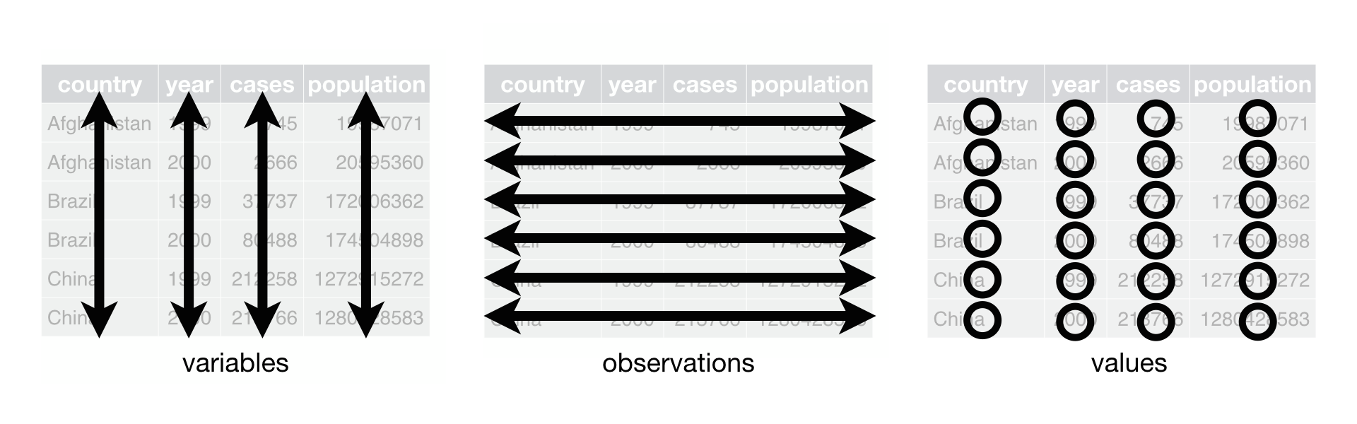
Figure from
Rfor Data Science by H. Wickham
![]()
Tidy - Why?
Why emphasize tidy data?
Minimize distractions:
- Free to focus on analysis not code
Once data is “tidy”, you can focus on the real questions
First goal for data pre-processing (“tidying up”)
Tidy - Who (and When)?
The name and principles of “tidy data” were popularized by H. Wickham (2014)
Core ideas are much older, dating back to (at least) Codd’s Relational Model in the 1970s, now ubiquitous in relational databases (SQL)
Now found in:
- Python (
pandas) - Julia (
DataFrames) - Rust (
polars) - and more
Tidy - How (and Where)?
tidyverse - Packages for Manipulating Tidy Data:
ggplot2: Visualizationdplyr:SQL-like operationstidyr: Reshaping and cleaning datareadr: Ingest tidy data intoR- Tidy manipulation of different data types:
stringr,forcats,lubridate
More helpers in the background (tibble, vctrs, …)
Aside: tibbles
You will sometimes see tibble (tbl_df) as a synonym for data.frame
- Minor differences in output formatting
- Fewer edge cases
Some Untidy Examples
Baruch college business core enrollment:
# A tibble: 6 × 4
  Semester Course     Enrollment   Cap
  <chr>    <chr>           <dbl> <dbl>
1 Fall     Accounting        200   250
2 Fall     Law               100   125
3 Fall     Statistics        200   200
4 Spring   Accounting        300   350
5 Spring   Law                50   100
6 Spring   Statistics        400   400
Tidy! ✅
- Each row is one unit (a class) 👍
- Columns are well-typed 👍
- One piece of information per column 👍
Some Untidy Examples
A different structure:
# A tibble: 6 × 3
  Semester Course     Enrollment
  <chr>    <chr>      <chr>
1 Fall     Accounting "200 of 250"
2 Fall     Law        "100 of 125"
3 Fall     Statistics "200 of 200"
4 Spring   Accounting "300 of 350"
5 Spring   Law        " 50 of 100"
6 Spring   Statistics "400 of 400"
Untidy! ❌
Multiple pieces of information per cell (Enrollment)
Some Untidy Examples
A different structure:
# A tibble: 12 × 4
   Semester Course     Number Type
   <chr>    <chr>       <dbl> <chr>
 1 Fall     Accounting    200 Enrollment
 2 Fall     Accounting    250 Cap
 3 Fall     Law           100 Enrollment
 4 Fall     Law           125 Cap
 5 Fall     Statistics    200 Enrollment
 6 Fall     Statistics    200 Cap
 7 Spring   Accounting    300 Enrollment
 8 Spring   Accounting    350 Cap
 9 Spring   Law            50 Enrollment
10 Spring   Law           100 Cap
11 Spring   Statistics    400 Enrollment
12 Spring   Statistics    400 Cap
Untidy! ❌
Mixing two pieces of information (Enrollments and Caps)
Tip: When one unit spans multiple rows, likely untidy
Some Untidy Examples
A different structure:
# A tibble: 6 × 3
  Semester Course     Enrollment
  <chr>    <chr>           <dbl>
1 Fall     Accounting        200
2 Fall     Law               100
3 Fall     Statistics        200
# ℹ 3 more rows
and
# A tibble: 6 × 3
  Semester Course       Cap
  <chr>    <chr>      <dbl>
1 Fall     Accounting   250
2 Fall     Law          125
3 Fall     Statistics   200
# ℹ 3 more rows
[A little bit] Untidy! ❌
Data spread across multiple tables - we will handle this next week
dplyr
The dplyr package exists for SQL-type manipulations of data.frames
Can load directly
library(dplyr)
or with the tidyverse meta-package
library(tidyverse)
tidyverse will give some messages about name conflicts - these are harmless
Data Frame Structure
Use the glimpse function to get a high-level summary of a data frame:
Rows: 344
Columns: 8
$ species     <fct> Adelie, Adelie, Adelie, Adelie, Adelie, Adelie, Adelie, Ad…
$ island      <fct> Torgersen, Torgersen, Torgersen, Torgersen, Torgersen, Tor…
$ bill_len    <dbl> 39.1, 39.5, 40.3, NA, 36.7, 39.3, 38.9, 39.2, 34.1, 42.0, …
$ bill_dep    <dbl> 18.7, 17.4, 18.0, NA, 19.3, 20.6, 17.8, 19.6, 18.1, 20.2, …
$ flipper_len <int> 181, 186, 195, NA, 193, 190, 181, 195, 193, 190, 186, 180,…
$ body_mass   <int> 3750, 3800, 3250, NA, 3450, 3650, 3625, 4675, 3475, 4250, …
$ sex         <fct> male, female, female, NA, female, male, female, male, NA, …
$ year        <int> 2007, 2007, 2007, 2007, 2007, 2007, 2007, 2007, 2007, 2007…
select and rename
How can we select certain columns?
select() will pick columns
      species    island bill_dep
1      Adelie Torgersen     18.7
2      Adelie Torgersen     17.4
3      Adelie Torgersen     18.0
4      Adelie Torgersen       NA
5      Adelie Torgersen     19.3
6      Adelie Torgersen     20.6
7      Adelie Torgersen     17.8
8      Adelie Torgersen     19.6
9      Adelie Torgersen     18.1
10     Adelie Torgersen     20.2
11     Adelie Torgersen     17.1
12     Adelie Torgersen     17.3
13     Adelie Torgersen     17.6
14     Adelie Torgersen     21.2
15     Adelie Torgersen     21.1
16     Adelie Torgersen     17.8
17     Adelie Torgersen     19.0
18     Adelie Torgersen     20.7
19     Adelie Torgersen     18.4
20     Adelie Torgersen     21.5
21     Adelie    Biscoe     18.3
22     Adelie    Biscoe     18.7
23     Adelie    Biscoe     19.2
24     Adelie    Biscoe     18.1
25     Adelie    Biscoe     17.2
26     Adelie    Biscoe     18.9
27     Adelie    Biscoe     18.6
28     Adelie    Biscoe     17.9
29     Adelie    Biscoe     18.6
30     Adelie    Biscoe     18.9
31     Adelie     Dream     16.7
32     Adelie     Dream     18.1
33     Adelie     Dream     17.8
34     Adelie     Dream     18.9
35     Adelie     Dream     17.0
36     Adelie     Dream     21.1
37     Adelie     Dream     20.0
38     Adelie     Dream     18.5
39     Adelie     Dream     19.3
40     Adelie     Dream     19.1
41     Adelie     Dream     18.0
42     Adelie     Dream     18.4
43     Adelie     Dream     18.5
44     Adelie     Dream     19.7
45     Adelie     Dream     16.9
46     Adelie     Dream     18.8
47     Adelie     Dream     19.0
48     Adelie     Dream     18.9
49     Adelie     Dream     17.9
50     Adelie     Dream     21.2
51     Adelie    Biscoe     17.7
52     Adelie    Biscoe     18.9
53     Adelie    Biscoe     17.9
54     Adelie    Biscoe     19.5
55     Adelie    Biscoe     18.1
56     Adelie    Biscoe     18.6
57     Adelie    Biscoe     17.5
58     Adelie    Biscoe     18.8
59     Adelie    Biscoe     16.6
60     Adelie    Biscoe     19.1
61     Adelie    Biscoe     16.9
62     Adelie    Biscoe     21.1
63     Adelie    Biscoe     17.0
64     Adelie    Biscoe     18.2
65     Adelie    Biscoe     17.1
66     Adelie    Biscoe     18.0
67     Adelie    Biscoe     16.2
68     Adelie    Biscoe     19.1
69     Adelie Torgersen     16.6
70     Adelie Torgersen     19.4
71     Adelie Torgersen     19.0
72     Adelie Torgersen     18.4
73     Adelie Torgersen     17.2
74     Adelie Torgersen     18.9
75     Adelie Torgersen     17.5
76     Adelie Torgersen     18.5
77     Adelie Torgersen     16.8
78     Adelie Torgersen     19.4
79     Adelie Torgersen     16.1
80     Adelie Torgersen     19.1
81     Adelie Torgersen     17.2
82     Adelie Torgersen     17.6
83     Adelie Torgersen     18.8
84     Adelie Torgersen     19.4
85     Adelie     Dream     17.8
86     Adelie     Dream     20.3
87     Adelie     Dream     19.5
88     Adelie     Dream     18.6
89     Adelie     Dream     19.2
90     Adelie     Dream     18.8
91     Adelie     Dream     18.0
92     Adelie     Dream     18.1
93     Adelie     Dream     17.1
94     Adelie     Dream     18.1
95     Adelie     Dream     17.3
96     Adelie     Dream     18.9
97     Adelie     Dream     18.6
98     Adelie     Dream     18.5
99     Adelie     Dream     16.1
100    Adelie     Dream     18.5
101    Adelie    Biscoe     17.9
102    Adelie    Biscoe     20.0
103    Adelie    Biscoe     16.0
104    Adelie    Biscoe     20.0
105    Adelie    Biscoe     18.6
106    Adelie    Biscoe     18.9
107    Adelie    Biscoe     17.2
108    Adelie    Biscoe     20.0
109    Adelie    Biscoe     17.0
110    Adelie    Biscoe     19.0
111    Adelie    Biscoe     16.5
112    Adelie    Biscoe     20.3
113    Adelie    Biscoe     17.7
114    Adelie    Biscoe     19.5
115    Adelie    Biscoe     20.7
116    Adelie    Biscoe     18.3
117    Adelie Torgersen     17.0
118    Adelie Torgersen     20.5
119    Adelie Torgersen     17.0
120    Adelie Torgersen     18.6
121    Adelie Torgersen     17.2
122    Adelie Torgersen     19.8
123    Adelie Torgersen     17.0
124    Adelie Torgersen     18.5
125    Adelie Torgersen     15.9
126    Adelie Torgersen     19.0
127    Adelie Torgersen     17.6
128    Adelie Torgersen     18.3
129    Adelie Torgersen     17.1
130    Adelie Torgersen     18.0
131    Adelie Torgersen     17.9
132    Adelie Torgersen     19.2
133    Adelie     Dream     18.5
134    Adelie     Dream     18.5
135    Adelie     Dream     17.6
136    Adelie     Dream     17.5
137    Adelie     Dream     17.5
138    Adelie     Dream     20.1
139    Adelie     Dream     16.5
140    Adelie     Dream     17.9
141    Adelie     Dream     17.1
142    Adelie     Dream     17.2
143    Adelie     Dream     15.5
144    Adelie     Dream     17.0
145    Adelie     Dream     16.8
146    Adelie     Dream     18.7
147    Adelie     Dream     18.6
148    Adelie     Dream     18.4
149    Adelie     Dream     17.8
150    Adelie     Dream     18.1
151    Adelie     Dream     17.1
152    Adelie     Dream     18.5
153    Gentoo    Biscoe     13.2
154    Gentoo    Biscoe     16.3
155    Gentoo    Biscoe     14.1
156    Gentoo    Biscoe     15.2
157    Gentoo    Biscoe     14.5
158    Gentoo    Biscoe     13.5
159    Gentoo    Biscoe     14.6
160    Gentoo    Biscoe     15.3
161    Gentoo    Biscoe     13.4
162    Gentoo    Biscoe     15.4
163    Gentoo    Biscoe     13.7
164    Gentoo    Biscoe     16.1
165    Gentoo    Biscoe     13.7
166    Gentoo    Biscoe     14.6
167    Gentoo    Biscoe     14.6
168    Gentoo    Biscoe     15.7
169    Gentoo    Biscoe     13.5
170    Gentoo    Biscoe     15.2
171    Gentoo    Biscoe     14.5
172    Gentoo    Biscoe     15.1
173    Gentoo    Biscoe     14.3
174    Gentoo    Biscoe     14.5
175    Gentoo    Biscoe     14.5
176    Gentoo    Biscoe     15.8
177    Gentoo    Biscoe     13.1
178    Gentoo    Biscoe     15.1
179    Gentoo    Biscoe     14.3
180    Gentoo    Biscoe     15.0
181    Gentoo    Biscoe     14.3
182    Gentoo    Biscoe     15.3
183    Gentoo    Biscoe     15.3
184    Gentoo    Biscoe     14.2
185    Gentoo    Biscoe     14.5
186    Gentoo    Biscoe     17.0
187    Gentoo    Biscoe     14.8
188    Gentoo    Biscoe     16.3
189    Gentoo    Biscoe     13.7
190    Gentoo    Biscoe     17.3
191    Gentoo    Biscoe     13.6
192    Gentoo    Biscoe     15.7
193    Gentoo    Biscoe     13.7
194    Gentoo    Biscoe     16.0
195    Gentoo    Biscoe     13.7
196    Gentoo    Biscoe     15.0
197    Gentoo    Biscoe     15.9
198    Gentoo    Biscoe     13.9
199    Gentoo    Biscoe     13.9
200    Gentoo    Biscoe     15.9
201    Gentoo    Biscoe     13.3
202    Gentoo    Biscoe     15.8
203    Gentoo    Biscoe     14.2
204    Gentoo    Biscoe     14.1
205    Gentoo    Biscoe     14.4
206    Gentoo    Biscoe     15.0
207    Gentoo    Biscoe     14.4
208    Gentoo    Biscoe     15.4
209    Gentoo    Biscoe     13.9
210    Gentoo    Biscoe     15.0
211    Gentoo    Biscoe     14.5
212    Gentoo    Biscoe     15.3
213    Gentoo    Biscoe     13.8
214    Gentoo    Biscoe     14.9
215    Gentoo    Biscoe     13.9
216    Gentoo    Biscoe     15.7
217    Gentoo    Biscoe     14.2
218    Gentoo    Biscoe     16.8
219    Gentoo    Biscoe     14.4
220    Gentoo    Biscoe     16.2
221    Gentoo    Biscoe     14.2
222    Gentoo    Biscoe     15.0
223    Gentoo    Biscoe     15.0
224    Gentoo    Biscoe     15.6
225    Gentoo    Biscoe     15.6
226    Gentoo    Biscoe     14.8
227    Gentoo    Biscoe     15.0
228    Gentoo    Biscoe     16.0
229    Gentoo    Biscoe     14.2
230    Gentoo    Biscoe     16.3
231    Gentoo    Biscoe     13.8
232    Gentoo    Biscoe     16.4
233    Gentoo    Biscoe     14.5
234    Gentoo    Biscoe     15.6
235    Gentoo    Biscoe     14.6
236    Gentoo    Biscoe     15.9
237    Gentoo    Biscoe     13.8
238    Gentoo    Biscoe     17.3
239    Gentoo    Biscoe     14.4
240    Gentoo    Biscoe     14.2
241    Gentoo    Biscoe     14.0
242    Gentoo    Biscoe     17.0
243    Gentoo    Biscoe     15.0
244    Gentoo    Biscoe     17.1
245    Gentoo    Biscoe     14.5
246    Gentoo    Biscoe     16.1
247    Gentoo    Biscoe     14.7
248    Gentoo    Biscoe     15.7
249    Gentoo    Biscoe     15.8
250    Gentoo    Biscoe     14.6
251    Gentoo    Biscoe     14.4
252    Gentoo    Biscoe     16.5
253    Gentoo    Biscoe     15.0
254    Gentoo    Biscoe     17.0
255    Gentoo    Biscoe     15.5
256    Gentoo    Biscoe     15.0
257    Gentoo    Biscoe     13.8
258    Gentoo    Biscoe     16.1
259    Gentoo    Biscoe     14.7
260    Gentoo    Biscoe     15.8
261    Gentoo    Biscoe     14.0
262    Gentoo    Biscoe     15.1
263    Gentoo    Biscoe     15.2
264    Gentoo    Biscoe     15.9
265    Gentoo    Biscoe     15.2
266    Gentoo    Biscoe     16.3
267    Gentoo    Biscoe     14.1
268    Gentoo    Biscoe     16.0
269    Gentoo    Biscoe     15.7
270    Gentoo    Biscoe     16.2
271    Gentoo    Biscoe     13.7
272    Gentoo    Biscoe       NA
273    Gentoo    Biscoe     14.3
274    Gentoo    Biscoe     15.7
275    Gentoo    Biscoe     14.8
276    Gentoo    Biscoe     16.1
277 Chinstrap     Dream     17.9
278 Chinstrap     Dream     19.5
279 Chinstrap     Dream     19.2
280 Chinstrap     Dream     18.7
281 Chinstrap     Dream     19.8
282 Chinstrap     Dream     17.8
283 Chinstrap     Dream     18.2
284 Chinstrap     Dream     18.2
285 Chinstrap     Dream     18.9
286 Chinstrap     Dream     19.9
287 Chinstrap     Dream     17.8
288 Chinstrap     Dream     20.3
289 Chinstrap     Dream     17.3
290 Chinstrap     Dream     18.1
291 Chinstrap     Dream     17.1
292 Chinstrap     Dream     19.6
293 Chinstrap     Dream     20.0
294 Chinstrap     Dream     17.8
295 Chinstrap     Dream     18.6
296 Chinstrap     Dream     18.2
297 Chinstrap     Dream     17.3
298 Chinstrap     Dream     17.5
299 Chinstrap     Dream     16.6
300 Chinstrap     Dream     19.4
301 Chinstrap     Dream     17.9
302 Chinstrap     Dream     19.0
303 Chinstrap     Dream     18.4
304 Chinstrap     Dream     19.0
305 Chinstrap     Dream     17.8
306 Chinstrap     Dream     20.0
307 Chinstrap     Dream     16.6
308 Chinstrap     Dream     20.8
309 Chinstrap     Dream     16.7
310 Chinstrap     Dream     18.8
311 Chinstrap     Dream     18.6
312 Chinstrap     Dream     16.8
313 Chinstrap     Dream     18.3
314 Chinstrap     Dream     20.7
315 Chinstrap     Dream     16.6
316 Chinstrap     Dream     19.9
317 Chinstrap     Dream     19.5
318 Chinstrap     Dream     17.5
319 Chinstrap     Dream     19.1
320 Chinstrap     Dream     17.0
321 Chinstrap     Dream     17.9
322 Chinstrap     Dream     18.5
323 Chinstrap     Dream     17.9
324 Chinstrap     Dream     19.6
325 Chinstrap     Dream     18.7
326 Chinstrap     Dream     17.3
327 Chinstrap     Dream     16.4
328 Chinstrap     Dream     19.0
329 Chinstrap     Dream     17.3
330 Chinstrap     Dream     19.7
331 Chinstrap     Dream     17.3
332 Chinstrap     Dream     18.8
333 Chinstrap     Dream     16.6
334 Chinstrap     Dream     19.9
335 Chinstrap     Dream     18.8
336 Chinstrap     Dream     19.4
337 Chinstrap     Dream     19.5
338 Chinstrap     Dream     16.5
339 Chinstrap     Dream     17.0
340 Chinstrap     Dream     19.8
341 Chinstrap     Dream     18.1
342 Chinstrap     Dream     18.2
343 Chinstrap     Dream     19.0
344 Chinstrap     Dream     18.7
Pipe Syntax
Pipe syntax (|>) is syntactic sugar - read as “and then”
Just makes code easier to read:
Exactly the same execution: improved UX
%>% is an older way of doing essentially the same thing - avoid it
Pipe Syntax
Pipe syntax is useful for longer multi-step operations:
Read top to bottom instead of inside out
select and rename
Can also use select to drop columns:
bill_len flipper_len body_mass sex year
1 39.1 181 3750 male 2007
2 39.5 186 3800 female 2007
3 40.3 195 3250 female 2007
4 NA NA NA <NA> 2007
5 36.7 193 3450 female 2007
6 39.3 190 3650 male 2007
7 38.9 181 3625 female 2007
8 39.2 195 4675 male 2007
9 34.1 193 3475 <NA> 2007
10 42.0 190 4250 <NA> 2007
11 37.8 186 3300 <NA> 2007
12 37.8 180 3700 <NA> 2007
13 41.1 182 3200 female 2007
14 38.6 191 3800 male 2007
15 34.6 198 4400 male 2007
16 36.6 185 3700 female 2007
17 38.7 195 3450 female 2007
18 42.5 197 4500 male 2007
19 34.4 184 3325 female 2007
20 46.0 194 4200 male 2007
21 37.8 174 3400 female 2007
22 37.7 180 3600 male 2007
23 35.9 189 3800 female 2007
24 38.2 185 3950 male 2007
25 38.8 180 3800 male 2007
26 35.3 187 3800 female 2007
27 40.6 183 3550 male 2007
28 40.5 187 3200 female 2007
29 37.9 172 3150 female 2007
30 40.5 180 3950 male 2007
31 39.5 178 3250 female 2007
32 37.2 178 3900 male 2007
33 39.5 188 3300 female 2007
34 40.9 184 3900 male 2007
35 36.4 195 3325 female 2007
36 39.2 196 4150 male 2007
37 38.8 190 3950 male 2007
38 42.2 180 3550 female 2007
39 37.6 181 3300 female 2007
40 39.8 184 4650 male 2007
41 36.5 182 3150 female 2007
42 40.8 195 3900 male 2007
43 36.0 186 3100 female 2007
44 44.1 196 4400 male 2007
45 37.0 185 3000 female 2007
46 39.6 190 4600 male 2007
47 41.1 182 3425 male 2007
48 37.5 179 2975 <NA> 2007
49 36.0 190 3450 female 2007
50 42.3 191 4150 male 2007
51 39.6 186 3500 female 2008
52 40.1 188 4300 male 2008
53 35.0 190 3450 female 2008
54 42.0 200 4050 male 2008
55 34.5 187 2900 female 2008
56 41.4 191 3700 male 2008
57 39.0 186 3550 female 2008
58 40.6 193 3800 male 2008
59 36.5 181 2850 female 2008
60 37.6 194 3750 male 2008
61 35.7 185 3150 female 2008
62 41.3 195 4400 male 2008
63 37.6 185 3600 female 2008
64 41.1 192 4050 male 2008
65 36.4 184 2850 female 2008
66 41.6 192 3950 male 2008
67 35.5 195 3350 female 2008
68 41.1 188 4100 male 2008
69 35.9 190 3050 female 2008
70 41.8 198 4450 male 2008
71 33.5 190 3600 female 2008
72 39.7 190 3900 male 2008
73 39.6 196 3550 female 2008
74 45.8 197 4150 male 2008
75 35.5 190 3700 female 2008
76 42.8 195 4250 male 2008
77 40.9 191 3700 female 2008
78 37.2 184 3900 male 2008
79 36.2 187 3550 female 2008
80 42.1 195 4000 male 2008
81 34.6 189 3200 female 2008
82 42.9 196 4700 male 2008
83 36.7 187 3800 female 2008
84 35.1 193 4200 male 2008
85 37.3 191 3350 female 2008
86 41.3 194 3550 male 2008
87 36.3 190 3800 male 2008
88 36.9 189 3500 female 2008
89 38.3 189 3950 male 2008
90 38.9 190 3600 female 2008
91 35.7 202 3550 female 2008
92 41.1 205 4300 male 2008
93 34.0 185 3400 female 2008
94 39.6 186 4450 male 2008
95 36.2 187 3300 female 2008
96 40.8 208 4300 male 2008
97 38.1 190 3700 female 2008
98 40.3 196 4350 male 2008
99 33.1 178 2900 female 2008
100 43.2 192 4100 male 2008
101 35.0 192 3725 female 2009
102 41.0 203 4725 male 2009
103 37.7 183 3075 female 2009
104 37.8 190 4250 male 2009
105 37.9 193 2925 female 2009
106 39.7 184 3550 male 2009
107 38.6 199 3750 female 2009
108 38.2 190 3900 male 2009
109 38.1 181 3175 female 2009
110 43.2 197 4775 male 2009
111 38.1 198 3825 female 2009
112 45.6 191 4600 male 2009
113 39.7 193 3200 female 2009
114 42.2 197 4275 male 2009
115 39.6 191 3900 female 2009
116 42.7 196 4075 male 2009
117 38.6 188 2900 female 2009
118 37.3 199 3775 male 2009
119 35.7 189 3350 female 2009
120 41.1 189 3325 male 2009
121 36.2 187 3150 female 2009
122 37.7 198 3500 male 2009
123 40.2 176 3450 female 2009
124 41.4 202 3875 male 2009
125 35.2 186 3050 female 2009
126 40.6 199 4000 male 2009
127 38.8 191 3275 female 2009
128 41.5 195 4300 male 2009
129 39.0 191 3050 female 2009
130 44.1 210 4000 male 2009
131 38.5 190 3325 female 2009
132 43.1 197 3500 male 2009
133 36.8 193 3500 female 2009
134 37.5 199 4475 male 2009
135 38.1 187 3425 female 2009
136 41.1 190 3900 male 2009
137 35.6 191 3175 female 2009
138 40.2 200 3975 male 2009
139 37.0 185 3400 female 2009
140 39.7 193 4250 male 2009
141 40.2 193 3400 female 2009
142 40.6 187 3475 male 2009
143 32.1 188 3050 female 2009
144 40.7 190 3725 male 2009
145 37.3 192 3000 female 2009
146 39.0 185 3650 male 2009
147 39.2 190 4250 male 2009
148 36.6 184 3475 female 2009
149 36.0 195 3450 female 2009
150 37.8 193 3750 male 2009
151 36.0 187 3700 female 2009
152 41.5 201 4000 male 2009
153 46.1 211 4500 female 2007
154 50.0 230 5700 male 2007
155 48.7 210 4450 female 2007
156 50.0 218 5700 male 2007
157 47.6 215 5400 male 2007
158 46.5 210 4550 female 2007
159 45.4 211 4800 female 2007
160 46.7 219 5200 male 2007
161 43.3 209 4400 female 2007
162 46.8 215 5150 male 2007
163 40.9 214 4650 female 2007
164 49.0 216 5550 male 2007
165 45.5 214 4650 female 2007
166 48.4 213 5850 male 2007
167 45.8 210 4200 female 2007
168 49.3 217 5850 male 2007
169 42.0 210 4150 female 2007
170 49.2 221 6300 male 2007
171 46.2 209 4800 female 2007
172 48.7 222 5350 male 2007
173 50.2 218 5700 male 2007
174 45.1 215 5000 female 2007
175 46.5 213 4400 female 2007
176 46.3 215 5050 male 2007
177 42.9 215 5000 female 2007
178 46.1 215 5100 male 2007
179 44.5 216 4100 <NA> 2007
180 47.8 215 5650 male 2007
181 48.2 210 4600 female 2007
182 50.0 220 5550 male 2007
183 47.3 222 5250 male 2007
184 42.8 209 4700 female 2007
185 45.1 207 5050 female 2007
186 59.6 230 6050 male 2007
187 49.1 220 5150 female 2008
188 48.4 220 5400 male 2008
189 42.6 213 4950 female 2008
190 44.4 219 5250 male 2008
191 44.0 208 4350 female 2008
192 48.7 208 5350 male 2008
193 42.7 208 3950 female 2008
194 49.6 225 5700 male 2008
195 45.3 210 4300 female 2008
196 49.6 216 4750 male 2008
197 50.5 222 5550 male 2008
198 43.6 217 4900 female 2008
199 45.5 210 4200 female 2008
200 50.5 225 5400 male 2008
201 44.9 213 5100 female 2008
202 45.2 215 5300 male 2008
203 46.6 210 4850 female 2008
204 48.5 220 5300 male 2008
205 45.1 210 4400 female 2008
206 50.1 225 5000 male 2008
207 46.5 217 4900 female 2008
208 45.0 220 5050 male 2008
209 43.8 208 4300 female 2008
210 45.5 220 5000 male 2008
211 43.2 208 4450 female 2008
212 50.4 224 5550 male 2008
213 45.3 208 4200 female 2008
214 46.2 221 5300 male 2008
215 45.7 214 4400 female 2008
216 54.3 231 5650 male 2008
217 45.8 219 4700 female 2008
218 49.8 230 5700 male 2008
219 46.2 214 4650 <NA> 2008
220 49.5 229 5800 male 2008
221 43.5 220 4700 female 2008
222 50.7 223 5550 male 2008
223 47.7 216 4750 female 2008
224 46.4 221 5000 male 2008
225 48.2 221 5100 male 2008
226 46.5 217 5200 female 2008
227 46.4 216 4700 female 2008
228 48.6 230 5800 male 2008
229 47.5 209 4600 female 2008
230 51.1 220 6000 male 2008
231 45.2 215 4750 female 2008
232 45.2 223 5950 male 2008
233 49.1 212 4625 female 2009
234 52.5 221 5450 male 2009
235 47.4 212 4725 female 2009
236 50.0 224 5350 male 2009
237 44.9 212 4750 female 2009
238 50.8 228 5600 male 2009
239 43.4 218 4600 female 2009
240 51.3 218 5300 male 2009
241 47.5 212 4875 female 2009
242 52.1 230 5550 male 2009
243 47.5 218 4950 female 2009
244 52.2 228 5400 male 2009
245 45.5 212 4750 female 2009
246 49.5 224 5650 male 2009
247 44.5 214 4850 female 2009
248 50.8 226 5200 male 2009
249 49.4 216 4925 male 2009
250 46.9 222 4875 female 2009
251 48.4 203 4625 female 2009
252 51.1 225 5250 male 2009
253 48.5 219 4850 female 2009
254 55.9 228 5600 male 2009
255 47.2 215 4975 female 2009
256 49.1 228 5500 male 2009
257 47.3 216 4725 <NA> 2009
258 46.8 215 5500 male 2009
259 41.7 210 4700 female 2009
260 53.4 219 5500 male 2009
261 43.3 208 4575 female 2009
262 48.1 209 5500 male 2009
263 50.5 216 5000 female 2009
264 49.8 229 5950 male 2009
265 43.5 213 4650 female 2009
266 51.5 230 5500 male 2009
267 46.2 217 4375 female 2009
268 55.1 230 5850 male 2009
269 44.5 217 4875 <NA> 2009
270 48.8 222 6000 male 2009
271 47.2 214 4925 female 2009
272 NA NA NA <NA> 2009
273 46.8 215 4850 female 2009
274 50.4 222 5750 male 2009
275 45.2 212 5200 female 2009
276 49.9 213 5400 male 2009
277 46.5 192 3500 female 2007
278 50.0 196 3900 male 2007
279 51.3 193 3650 male 2007
280 45.4 188 3525 female 2007
281 52.7 197 3725 male 2007
282 45.2 198 3950 female 2007
283 46.1 178 3250 female 2007
284 51.3 197 3750 male 2007
285 46.0 195 4150 female 2007
286 51.3 198 3700 male 2007
287 46.6 193 3800 female 2007
288 51.7 194 3775 male 2007
289 47.0 185 3700 female 2007
290 52.0 201 4050 male 2007
291 45.9 190 3575 female 2007
292 50.5 201 4050 male 2007
293 50.3 197 3300 male 2007
294 58.0 181 3700 female 2007
295 46.4 190 3450 female 2007
296 49.2 195 4400 male 2007
297 42.4 181 3600 female 2007
298 48.5 191 3400 male 2007
299 43.2 187 2900 female 2007
300 50.6 193 3800 male 2007
301 46.7 195 3300 female 2007
302 52.0 197 4150 male 2007
303 50.5 200 3400 female 2008
304 49.5 200 3800 male 2008
305 46.4 191 3700 female 2008
306 52.8 205 4550 male 2008
307 40.9 187 3200 female 2008
308 54.2 201 4300 male 2008
309 42.5 187 3350 female 2008
310 51.0 203 4100 male 2008
311 49.7 195 3600 male 2008
312 47.5 199 3900 female 2008
313 47.6 195 3850 female 2008
314 52.0 210 4800 male 2008
315 46.9 192 2700 female 2008
316 53.5 205 4500 male 2008
317 49.0 210 3950 male 2008
318 46.2 187 3650 female 2008
319 50.9 196 3550 male 2008
320 45.5 196 3500 female 2008
321 50.9 196 3675 female 2009
322 50.8 201 4450 male 2009
323 50.1 190 3400 female 2009
324 49.0 212 4300 male 2009
325 51.5 187 3250 male 2009
326 49.8 198 3675 female 2009
327 48.1 199 3325 female 2009
328 51.4 201 3950 male 2009
329 45.7 193 3600 female 2009
330 50.7 203 4050 male 2009
331 42.5 187 3350 female 2009
332 52.2 197 3450 male 2009
333 45.2 191 3250 female 2009
334 49.3 203 4050 male 2009
335 50.2 202 3800 male 2009
336 45.6 194 3525 female 2009
337 51.9 206 3950 male 2009
338 46.8 189 3650 female 2009
339 45.7 195 3650 female 2009
340 55.8 207 4000 male 2009
341 43.5 202 3400 female 2009
342 49.6 193 3775 male 2009
343 50.8 210 4100 male 2009
344 50.2 198 3775 female 2009select and rename
You can but shouldn’t mix select and drop - results non-intuitive
      species
1      Adelie
2      Adelie
3      Adelie
4      Adelie
5      Adelie
6      Adelie
7      Adelie
8      Adelie
9      Adelie
10     Adelie
11     Adelie
12     Adelie
13     Adelie
14     Adelie
15     Adelie
16     Adelie
17     Adelie
18     Adelie
19     Adelie
20     Adelie
21     Adelie
22     Adelie
23     Adelie
24     Adelie
25     Adelie
26     Adelie
27     Adelie
28     Adelie
29     Adelie
30     Adelie
31     Adelie
32     Adelie
33     Adelie
34     Adelie
35     Adelie
36     Adelie
37     Adelie
38     Adelie
39     Adelie
40     Adelie
41     Adelie
42     Adelie
43     Adelie
44     Adelie
45     Adelie
46     Adelie
47     Adelie
48     Adelie
49     Adelie
50     Adelie
51     Adelie
52     Adelie
53     Adelie
54     Adelie
55     Adelie
56     Adelie
57     Adelie
58     Adelie
59     Adelie
60     Adelie
61     Adelie
62     Adelie
63     Adelie
64     Adelie
65     Adelie
66     Adelie
67     Adelie
68     Adelie
69     Adelie
70     Adelie
71     Adelie
72     Adelie
73     Adelie
74     Adelie
75     Adelie
76     Adelie
77     Adelie
78     Adelie
79     Adelie
80     Adelie
81     Adelie
82     Adelie
83     Adelie
84     Adelie
85     Adelie
86     Adelie
87     Adelie
88     Adelie
89     Adelie
90     Adelie
91     Adelie
92     Adelie
93     Adelie
94     Adelie
95     Adelie
96     Adelie
97     Adelie
98     Adelie
99     Adelie
100    Adelie
101    Adelie
102    Adelie
103    Adelie
104    Adelie
105    Adelie
106    Adelie
107    Adelie
108    Adelie
109    Adelie
110    Adelie
111    Adelie
112    Adelie
113    Adelie
114    Adelie
115    Adelie
116    Adelie
117    Adelie
118    Adelie
119    Adelie
120    Adelie
121    Adelie
122    Adelie
123    Adelie
124    Adelie
125    Adelie
126    Adelie
127    Adelie
128    Adelie
129    Adelie
130    Adelie
131    Adelie
132    Adelie
133    Adelie
134    Adelie
135    Adelie
136    Adelie
137    Adelie
138    Adelie
139    Adelie
140    Adelie
141    Adelie
142    Adelie
143    Adelie
144    Adelie
145    Adelie
146    Adelie
147    Adelie
148    Adelie
149    Adelie
150    Adelie
151    Adelie
152    Adelie
153    Gentoo
154    Gentoo
155    Gentoo
156    Gentoo
157    Gentoo
158    Gentoo
159    Gentoo
160    Gentoo
161    Gentoo
162    Gentoo
163    Gentoo
164    Gentoo
165    Gentoo
166    Gentoo
167    Gentoo
168    Gentoo
169    Gentoo
170    Gentoo
171    Gentoo
172    Gentoo
173    Gentoo
174    Gentoo
175    Gentoo
176    Gentoo
177    Gentoo
178    Gentoo
179    Gentoo
180    Gentoo
181    Gentoo
182    Gentoo
183    Gentoo
184    Gentoo
185    Gentoo
186    Gentoo
187    Gentoo
188    Gentoo
189    Gentoo
190    Gentoo
191    Gentoo
192    Gentoo
193    Gentoo
194    Gentoo
195    Gentoo
196    Gentoo
197    Gentoo
198    Gentoo
199    Gentoo
200    Gentoo
201    Gentoo
202    Gentoo
203    Gentoo
204    Gentoo
205    Gentoo
206    Gentoo
207    Gentoo
208    Gentoo
209    Gentoo
210    Gentoo
211    Gentoo
212    Gentoo
213    Gentoo
214    Gentoo
215    Gentoo
216    Gentoo
217    Gentoo
218    Gentoo
219    Gentoo
220    Gentoo
221    Gentoo
222    Gentoo
223    Gentoo
224    Gentoo
225    Gentoo
226    Gentoo
227    Gentoo
228    Gentoo
229    Gentoo
230    Gentoo
231    Gentoo
232    Gentoo
233    Gentoo
234    Gentoo
235    Gentoo
236    Gentoo
237    Gentoo
238    Gentoo
239    Gentoo
240    Gentoo
241    Gentoo
242    Gentoo
243    Gentoo
244    Gentoo
245    Gentoo
246    Gentoo
247    Gentoo
248    Gentoo
249    Gentoo
250    Gentoo
251    Gentoo
252    Gentoo
253    Gentoo
254    Gentoo
255    Gentoo
256    Gentoo
257    Gentoo
258    Gentoo
259    Gentoo
260    Gentoo
261    Gentoo
262    Gentoo
263    Gentoo
264    Gentoo
265    Gentoo
266    Gentoo
267    Gentoo
268    Gentoo
269    Gentoo
270    Gentoo
271    Gentoo
272    Gentoo
273    Gentoo
274    Gentoo
275    Gentoo
276    Gentoo
277 Chinstrap
278 Chinstrap
279 Chinstrap
280 Chinstrap
281 Chinstrap
282 Chinstrap
283 Chinstrap
284 Chinstrap
285 Chinstrap
286 Chinstrap
287 Chinstrap
288 Chinstrap
289 Chinstrap
290 Chinstrap
291 Chinstrap
292 Chinstrap
293 Chinstrap
294 Chinstrap
295 Chinstrap
296 Chinstrap
297 Chinstrap
298 Chinstrap
299 Chinstrap
300 Chinstrap
301 Chinstrap
302 Chinstrap
303 Chinstrap
304 Chinstrap
305 Chinstrap
306 Chinstrap
307 Chinstrap
308 Chinstrap
309 Chinstrap
310 Chinstrap
311 Chinstrap
312 Chinstrap
313 Chinstrap
314 Chinstrap
315 Chinstrap
316 Chinstrap
317 Chinstrap
318 Chinstrap
319 Chinstrap
320 Chinstrap
321 Chinstrap
322 Chinstrap
323 Chinstrap
324 Chinstrap
325 Chinstrap
326 Chinstrap
327 Chinstrap
328 Chinstrap
329 Chinstrap
330 Chinstrap
331 Chinstrap
332 Chinstrap
333 Chinstrap
334 Chinstrap
335 Chinstrap
336 Chinstrap
337 Chinstrap
338 Chinstrap
339 Chinstrap
340 Chinstrap
341 Chinstrap
342 Chinstrap
343 Chinstrap
344 Chinstrap
select and rename
To avoid printing too much, let’s take a smaller subset of rows:
tidyselect
dplyr has many more selection functions for getting groups of related columns
See tidyselect for details
Creating Columns
The mutate command can be used to create new columns from old:
Named Arguments
mutate (and later summarize) create new columns:
mutatecreates “one-to-one”summarizecreates “one-per-group”
If you want to name them (so you can use them later), use named argument
Named Arguments
Default name is tricky to use:
  species    island bill_len bill_dep flipper_len body_mass year n()
1  Adelie Torgersen     39.1     18.7         181      3750 2007   5
2  Adelie Torgersen     39.5     17.4         186      3800 2007   5
3  Adelie Torgersen     40.3     18.0         195      3250 2007   5
4  Adelie Torgersen       NA       NA          NA        NA 2007   5
5  Adelie Torgersen     36.7     19.3         193      3450 2007   5
vs
  species    island bill_len bill_dep flipper_len body_mass year n_penguins
1  Adelie Torgersen     39.1     18.7         181      3750 2007          5
2  Adelie Torgersen     39.5     17.4         186      3800 2007          5
3  Adelie Torgersen     40.3     18.0         195      3250 2007          5
4  Adelie Torgersen       NA       NA          NA        NA 2007          5
5  Adelie Torgersen     36.7     19.3         193      3450 2007          5
Provide a “valid” variable name for easiest use (alphanumeric, no punctuation other than _, starts with a letter)
mutate
Can create and use variables in order with mutate:
five_penguins |>
  select(body_mass, flipper_len, sex) |>
  mutate(body_mass_kg = body_mass / 1000,
         flipper_len_m = flipper_len / 1000,
         penguin_bmi = body_mass_kg / flipper_len_m^2)
body_mass flipper_len sex body_mass_kg flipper_len_m penguin_bmi
1 3750 181 male 3.75 0.181 114.46537
2 3800 186 female 3.80 0.186 109.83929
3 3250 195 female 3.25 0.195 85.47009
4 NA NA <NA> NA NA NA
5 3450 193 female 3.45 0.193 92.61994BMI probably isn’t accurate for penguins
mutate
Image from jgoode.com
mutate
Variables are created in order (top to bottom) - this fails:
five_penguins |>
  select(body_mass, flipper_len, sex) |>
  mutate(penguin_bmi = body_mass_kg / flipper_len_m^2,
         body_mass_kg = body_mass / 1000,
         flipper_len_m = flipper_len / 1000)
Error in `mutate()`:
ℹ In argument: `penguin_bmi = body_mass_kg/flipper_len_m^2`.
Caused by error:
! object 'body_mass_kg' not foundmutate helpers
Helper functions for working with complex mutate commands:
five_penguins |>
  select(body_mass, flipper_len, sex) |>
  mutate(body_mass_kg = body_mass / 1000,
         flipper_len_m = flipper_len / 1000,
         penguin_bmi = body_mass_kg / flipper_len_m^2,
         is_husky = if_else(penguin_bmi > 120, TRUE, FALSE))
body_mass flipper_len sex body_mass_kg flipper_len_m penguin_bmi is_husky
1 3750 181 male 3.75 0.181 114.46537 FALSE
2 3800 186 female 3.80 0.186 109.83929 FALSE
3 3250 195 female 3.25 0.195 85.47009 FALSE
4 NA NA <NA> NA NA NA NA
5 3450 193 female 3.45 0.193 92.61994 FALSEVectorized analogue of the if/else conditional construct
mutate helpers
case_when for multiple conditions:
five_penguins |> select(body_mass, flipper_len, sex) |>
  mutate(body_mass_kg = body_mass / 1000,
         flipper_len_m = flipper_len / 1000,
         penguin_bmi = body_mass_kg / flipper_len_m^2,
         is_big_guy = case_when(
           sex == "female" ~ FALSE,
           penguin_bmi < 120 ~ FALSE,
           .default = TRUE))
body_mass flipper_len sex body_mass_kg flipper_len_m penguin_bmi
1 3750 181 male 3.75 0.181 114.46537
2 3800 186 female 3.80 0.186 109.83929
3 3250 195 female 3.25 0.195 85.47009
4 NA NA <NA> NA NA NA
5 3450 193 female 3.45 0.193 92.61994
is_big_guy
1 FALSE
2 FALSE
3 FALSE
4 TRUE
5 FALSEDefines a sequence of tests: first to pass takes value from RHS of ~
mutate helpers
More advanced helpers for recoding and replacing in dplyr v1.2 (February 2026)
case_whenreplace_whenrecode_valuesreplace_valuesSee announcement for more details
filter Operations
While select is used to isolate columns, filter is used to isolate rows:
    species    island bill_len bill_dep flipper_len body_mass    sex year
1    Adelie Torgersen     39.1     18.7         181      3750   male 2007
2    Adelie Torgersen     39.5     17.4         186      3800 female 2007
3    Adelie Torgersen     40.3     18.0         195      3250 female 2007
4    Adelie Torgersen       NA       NA          NA        NA   <NA> 2007
5    Adelie Torgersen     36.7     19.3         193      3450 female 2007
6    Adelie Torgersen     39.3     20.6         190      3650   male 2007
7    Adelie Torgersen     38.9     17.8         181      3625 female 2007
8    Adelie Torgersen     39.2     19.6         195      4675   male 2007
9    Adelie Torgersen     34.1     18.1         193      3475   <NA> 2007
10   Adelie Torgersen     42.0     20.2         190      4250   <NA> 2007
11   Adelie Torgersen     37.8     17.1         186      3300   <NA> 2007
12   Adelie Torgersen     37.8     17.3         180      3700   <NA> 2007
13   Adelie Torgersen     41.1     17.6         182      3200 female 2007
14   Adelie Torgersen     38.6     21.2         191      3800   male 2007
15   Adelie Torgersen     34.6     21.1         198      4400   male 2007
16   Adelie Torgersen     36.6     17.8         185      3700 female 2007
17   Adelie Torgersen     38.7     19.0         195      3450 female 2007
18   Adelie Torgersen     42.5     20.7         197      4500   male 2007
19   Adelie Torgersen     34.4     18.4         184      3325 female 2007
20   Adelie Torgersen     46.0     21.5         194      4200   male 2007
21   Adelie    Biscoe     37.8     18.3         174      3400 female 2007
22   Adelie    Biscoe     37.7     18.7         180      3600   male 2007
23   Adelie    Biscoe     35.9     19.2         189      3800 female 2007
24   Adelie    Biscoe     38.2     18.1         185      3950   male 2007
25   Adelie    Biscoe     38.8     17.2         180      3800   male 2007
26   Adelie    Biscoe     35.3     18.9         187      3800 female 2007
27   Adelie    Biscoe     40.6     18.6         183      3550   male 2007
28   Adelie    Biscoe     40.5     17.9         187      3200 female 2007
29   Adelie    Biscoe     37.9     18.6         172      3150 female 2007
30   Adelie    Biscoe     40.5     18.9         180      3950   male 2007
31   Adelie     Dream     39.5     16.7         178      3250 female 2007
32   Adelie     Dream     37.2     18.1         178      3900   male 2007
33   Adelie     Dream     39.5     17.8         188      3300 female 2007
34   Adelie     Dream     40.9     18.9         184      3900   male 2007
35   Adelie     Dream     36.4     17.0         195      3325 female 2007
36   Adelie     Dream     39.2     21.1         196      4150   male 2007
37   Adelie     Dream     38.8     20.0         190      3950   male 2007
38   Adelie     Dream     42.2     18.5         180      3550 female 2007
39   Adelie     Dream     37.6     19.3         181      3300 female 2007
40   Adelie     Dream     39.8     19.1         184      4650   male 2007
41   Adelie     Dream     36.5     18.0         182      3150 female 2007
42   Adelie     Dream     40.8     18.4         195      3900   male 2007
43   Adelie     Dream     36.0     18.5         186      3100 female 2007
44   Adelie     Dream     44.1     19.7         196      4400   male 2007
45   Adelie     Dream     37.0     16.9         185      3000 female 2007
46   Adelie     Dream     39.6     18.8         190      4600   male 2007
47   Adelie     Dream     41.1     19.0         182      3425   male 2007
48   Adelie     Dream     37.5     18.9         179      2975   <NA> 2007
49   Adelie     Dream     36.0     17.9         190      3450 female 2007
50   Adelie     Dream     42.3     21.2         191      4150   male 2007
51   Adelie    Biscoe     39.6     17.7         186      3500 female 2008
52   Adelie    Biscoe     40.1     18.9         188      4300   male 2008
53   Adelie    Biscoe     35.0     17.9         190      3450 female 2008
54   Adelie    Biscoe     42.0     19.5         200      4050   male 2008
55   Adelie    Biscoe     34.5     18.1         187      2900 female 2008
56   Adelie    Biscoe     41.4     18.6         191      3700   male 2008
57   Adelie    Biscoe     39.0     17.5         186      3550 female 2008
58   Adelie    Biscoe     40.6     18.8         193      3800   male 2008
59   Adelie    Biscoe     36.5     16.6         181      2850 female 2008
60   Adelie    Biscoe     37.6     19.1         194      3750   male 2008
61   Adelie    Biscoe     35.7     16.9         185      3150 female 2008
62   Adelie    Biscoe     41.3     21.1         195      4400   male 2008
63   Adelie    Biscoe     37.6     17.0         185      3600 female 2008
64   Adelie    Biscoe     41.1     18.2         192      4050   male 2008
65   Adelie    Biscoe     36.4     17.1         184      2850 female 2008
66   Adelie    Biscoe     41.6     18.0         192      3950   male 2008
67   Adelie    Biscoe     35.5     16.2         195      3350 female 2008
68   Adelie    Biscoe     41.1     19.1         188      4100   male 2008
69   Adelie Torgersen     35.9     16.6         190      3050 female 2008
70   Adelie Torgersen     41.8     19.4         198      4450   male 2008
71   Adelie Torgersen     33.5     19.0         190      3600 female 2008
72   Adelie Torgersen     39.7     18.4         190      3900   male 2008
73   Adelie Torgersen     39.6     17.2         196      3550 female 2008
74   Adelie Torgersen     45.8     18.9         197      4150   male 2008
75   Adelie Torgersen     35.5     17.5         190      3700 female 2008
76   Adelie Torgersen     42.8     18.5         195      4250   male 2008
77   Adelie Torgersen     40.9     16.8         191      3700 female 2008
78   Adelie Torgersen     37.2     19.4         184      3900   male 2008
79   Adelie Torgersen     36.2     16.1         187      3550 female 2008
80   Adelie Torgersen     42.1     19.1         195      4000   male 2008
81   Adelie Torgersen     34.6     17.2         189      3200 female 2008
82   Adelie Torgersen     42.9     17.6         196      4700   male 2008
83   Adelie Torgersen     36.7     18.8         187      3800 female 2008
84   Adelie Torgersen     35.1     19.4         193      4200   male 2008
85   Adelie     Dream     37.3     17.8         191      3350 female 2008
86   Adelie     Dream     41.3     20.3         194      3550   male 2008
87   Adelie     Dream     36.3     19.5         190      3800   male 2008
88   Adelie     Dream     36.9     18.6         189      3500 female 2008
89   Adelie     Dream     38.3     19.2         189      3950   male 2008
90   Adelie     Dream     38.9     18.8         190      3600 female 2008
91   Adelie     Dream     35.7     18.0         202      3550 female 2008
92   Adelie     Dream     41.1     18.1         205      4300   male 2008
93   Adelie     Dream     34.0     17.1         185      3400 female 2008
94   Adelie     Dream     39.6     18.1         186      4450   male 2008
95   Adelie     Dream     36.2     17.3         187      3300 female 2008
96   Adelie     Dream     40.8     18.9         208      4300   male 2008
97   Adelie     Dream     38.1     18.6         190      3700 female 2008
98   Adelie     Dream     40.3     18.5         196      4350   male 2008
99   Adelie     Dream     33.1     16.1         178      2900 female 2008
100  Adelie     Dream     43.2     18.5         192      4100   male 2008
101  Adelie    Biscoe     35.0     17.9         192      3725 female 2009
102  Adelie    Biscoe     41.0     20.0         203      4725   male 2009
103  Adelie    Biscoe     37.7     16.0         183      3075 female 2009
104  Adelie    Biscoe     37.8     20.0         190      4250   male 2009
105  Adelie    Biscoe     37.9     18.6         193      2925 female 2009
106  Adelie    Biscoe     39.7     18.9         184      3550   male 2009
107  Adelie    Biscoe     38.6     17.2         199      3750 female 2009
108  Adelie    Biscoe     38.2     20.0         190      3900   male 2009
109  Adelie    Biscoe     38.1     17.0         181      3175 female 2009
110  Adelie    Biscoe     43.2     19.0         197      4775   male 2009
111  Adelie    Biscoe     38.1     16.5         198      3825 female 2009
112  Adelie    Biscoe     45.6     20.3         191      4600   male 2009
113  Adelie    Biscoe     39.7     17.7         193      3200 female 2009
114  Adelie    Biscoe     42.2     19.5         197      4275   male 2009
115  Adelie    Biscoe     39.6     20.7         191      3900 female 2009
116  Adelie    Biscoe     42.7     18.3         196      4075   male 2009
117  Adelie Torgersen     38.6     17.0         188      2900 female 2009
118  Adelie Torgersen     37.3     20.5         199      3775   male 2009
119  Adelie Torgersen     35.7     17.0         189      3350 female 2009
120  Adelie Torgersen     41.1     18.6         189      3325   male 2009
121  Adelie Torgersen     36.2     17.2         187      3150 female 2009
122  Adelie Torgersen     37.7     19.8         198      3500   male 2009
123  Adelie Torgersen     40.2     17.0         176      3450 female 2009
124  Adelie Torgersen     41.4     18.5         202      3875   male 2009
125  Adelie Torgersen     35.2     15.9         186      3050 female 2009
126  Adelie Torgersen     40.6     19.0         199      4000   male 2009
127  Adelie Torgersen     38.8     17.6         191      3275 female 2009
128  Adelie Torgersen     41.5     18.3         195      4300   male 2009
129  Adelie Torgersen     39.0     17.1         191      3050 female 2009
130  Adelie Torgersen     44.1     18.0         210      4000   male 2009
131  Adelie Torgersen     38.5     17.9         190      3325 female 2009
132  Adelie Torgersen     43.1     19.2         197      3500   male 2009
133  Adelie     Dream     36.8     18.5         193      3500 female 2009
134  Adelie     Dream     37.5     18.5         199      4475   male 2009
135  Adelie     Dream     38.1     17.6         187      3425 female 2009
136  Adelie     Dream     41.1     17.5         190      3900   male 2009
137  Adelie     Dream     35.6     17.5         191      3175 female 2009
138  Adelie     Dream     40.2     20.1         200      3975   male 2009
139  Adelie     Dream     37.0     16.5         185      3400 female 2009
140  Adelie     Dream     39.7     17.9         193      4250   male 2009
141  Adelie     Dream     40.2     17.1         193      3400 female 2009
142  Adelie     Dream     40.6     17.2         187      3475   male 2009
143  Adelie     Dream     32.1     15.5         188      3050 female 2009
144  Adelie     Dream     40.7     17.0         190      3725   male 2009
145  Adelie     Dream     37.3     16.8         192      3000 female 2009
146  Adelie     Dream     39.0     18.7         185      3650   male 2009
147  Adelie     Dream     39.2     18.6         190      4250   male 2009
148  Adelie     Dream     36.6     18.4         184      3475 female 2009
149  Adelie     Dream     36.0     17.8         195      3450 female 2009
150  Adelie     Dream     37.8     18.1         193      3750   male 2009
151  Adelie     Dream     36.0     17.1         187      3700 female 2009
152  Adelie     Dream     41.5     18.5         201      4000   male 2009
filter Operations
Pass multiple arguments to get the intersection
   species island bill_len bill_dep flipper_len body_mass    sex year
1   Adelie Biscoe     37.8     18.3         174      3400 female 2007
2   Adelie Biscoe     37.7     18.7         180      3600   male 2007
3   Adelie Biscoe     35.9     19.2         189      3800 female 2007
4   Adelie Biscoe     38.2     18.1         185      3950   male 2007
5   Adelie Biscoe     38.8     17.2         180      3800   male 2007
6   Adelie Biscoe     35.3     18.9         187      3800 female 2007
7   Adelie Biscoe     40.6     18.6         183      3550   male 2007
8   Adelie Biscoe     40.5     17.9         187      3200 female 2007
9   Adelie Biscoe     37.9     18.6         172      3150 female 2007
10  Adelie Biscoe     40.5     18.9         180      3950   male 2007
11  Adelie Biscoe     39.6     17.7         186      3500 female 2008
12  Adelie Biscoe     40.1     18.9         188      4300   male 2008
13  Adelie Biscoe     35.0     17.9         190      3450 female 2008
14  Adelie Biscoe     42.0     19.5         200      4050   male 2008
15  Adelie Biscoe     34.5     18.1         187      2900 female 2008
16  Adelie Biscoe     41.4     18.6         191      3700   male 2008
17  Adelie Biscoe     39.0     17.5         186      3550 female 2008
18  Adelie Biscoe     40.6     18.8         193      3800   male 2008
19  Adelie Biscoe     36.5     16.6         181      2850 female 2008
20  Adelie Biscoe     37.6     19.1         194      3750   male 2008
21  Adelie Biscoe     35.7     16.9         185      3150 female 2008
22  Adelie Biscoe     41.3     21.1         195      4400   male 2008
23  Adelie Biscoe     37.6     17.0         185      3600 female 2008
24  Adelie Biscoe     41.1     18.2         192      4050   male 2008
25  Adelie Biscoe     36.4     17.1         184      2850 female 2008
26  Adelie Biscoe     41.6     18.0         192      3950   male 2008
27  Adelie Biscoe     35.5     16.2         195      3350 female 2008
28  Adelie Biscoe     41.1     19.1         188      4100   male 2008
29  Adelie Biscoe     35.0     17.9         192      3725 female 2009
30  Adelie Biscoe     41.0     20.0         203      4725   male 2009
31  Adelie Biscoe     37.7     16.0         183      3075 female 2009
32  Adelie Biscoe     37.8     20.0         190      4250   male 2009
33  Adelie Biscoe     37.9     18.6         193      2925 female 2009
34  Adelie Biscoe     39.7     18.9         184      3550   male 2009
35  Adelie Biscoe     38.6     17.2         199      3750 female 2009
36  Adelie Biscoe     38.2     20.0         190      3900   male 2009
37  Adelie Biscoe     38.1     17.0         181      3175 female 2009
38  Adelie Biscoe     43.2     19.0         197      4775   male 2009
39  Adelie Biscoe     38.1     16.5         198      3825 female 2009
40  Adelie Biscoe     45.6     20.3         191      4600   male 2009
41  Adelie Biscoe     39.7     17.7         193      3200 female 2009
42  Adelie Biscoe     42.2     19.5         197      4275   male 2009
43  Adelie Biscoe     39.6     20.7         191      3900 female 2009
44  Adelie Biscoe     42.7     18.3         196      4075   male 2009
filter Operations
Can compute quantities inside of filter
To select heavier than average penguins:
  species    island bill_len bill_dep flipper_len body_mass    sex year
1  Adelie Torgersen     39.1     18.7         181      3750   male 2007
2  Adelie Torgersen     39.5     17.4         186      3800 female 2007
Reminder: Why do we need na.rm=TRUE?
slice_min and slice_max
The slice_min and slice_max functions replace and extend the common filter(x == max(x)) idiom:
slice_min and slice_max
Arguments:
n: How many rows to return (top/bottom \(k\))prop: Percent of rows to return
E.g., 10% lightest
     species    island bill_len bill_dep flipper_len body_mass    sex year
1  Chinstrap     Dream     46.9     16.6         192      2700 female 2008
2     Adelie    Biscoe     36.5     16.6         181      2850 female 2008
3     Adelie    Biscoe     36.4     17.1         184      2850 female 2008
4     Adelie    Biscoe     34.5     18.1         187      2900 female 2008
5     Adelie     Dream     33.1     16.1         178      2900 female 2008
6     Adelie Torgersen     38.6     17.0         188      2900 female 2009
7  Chinstrap     Dream     43.2     16.6         187      2900 female 2007
8     Adelie    Biscoe     37.9     18.6         193      2925 female 2009
9     Adelie     Dream     37.5     18.9         179      2975   <NA> 2007
10    Adelie     Dream     37.0     16.9         185      3000 female 2007
11    Adelie     Dream     37.3     16.8         192      3000 female 2009
12    Adelie Torgersen     35.9     16.6         190      3050 female 2008
13    Adelie Torgersen     35.2     15.9         186      3050 female 2009
14    Adelie Torgersen     39.0     17.1         191      3050 female 2009
15    Adelie     Dream     32.1     15.5         188      3050 female 2009
16    Adelie    Biscoe     37.7     16.0         183      3075 female 2009
17    Adelie     Dream     36.0     18.5         186      3100 female 2007
18    Adelie    Biscoe     37.9     18.6         172      3150 female 2007
19    Adelie     Dream     36.5     18.0         182      3150 female 2007
20    Adelie    Biscoe     35.7     16.9         185      3150 female 2008
21    Adelie Torgersen     36.2     17.2         187      3150 female 2009
22    Adelie    Biscoe     38.1     17.0         181      3175 female 2009
23    Adelie     Dream     35.6     17.5         191      3175 female 2009
24    Adelie Torgersen     41.1     17.6         182      3200 female 2007
25    Adelie    Biscoe     40.5     17.9         187      3200 female 2007
26    Adelie Torgersen     34.6     17.2         189      3200 female 2008
27    Adelie    Biscoe     39.7     17.7         193      3200 female 2009
28 Chinstrap     Dream     40.9     16.6         187      3200 female 2008
29    Adelie Torgersen     40.3     18.0         195      3250 female 2007
30    Adelie     Dream     39.5     16.7         178      3250 female 2007
31 Chinstrap     Dream     46.1     18.2         178      3250 female 2007
32 Chinstrap     Dream     51.5     18.7         187      3250   male 2009
33 Chinstrap     Dream     45.2     16.6         191      3250 female 2009
34    Adelie Torgersen     38.8     17.6         191      3275 female 2009
slice_sample
slice_sample generates a random subset:
- Useful for getting a smaller and faster “exploratory set”
     species    island bill_len bill_dep flipper_len body_mass    sex year
1     Gentoo    Biscoe     50.5     15.9         225      5400   male 2008
2     Adelie     Dream     36.3     19.5         190      3800   male 2008
3     Adelie     Dream     36.6     18.4         184      3475 female 2009
4     Gentoo    Biscoe     45.4     14.6         211      4800 female 2007
5     Adelie    Biscoe     41.1     18.2         192      4050   male 2008
6     Gentoo    Biscoe     48.6     16.0         230      5800   male 2008
7     Gentoo    Biscoe     43.8     13.9         208      4300 female 2008
8     Gentoo    Biscoe     44.5     15.7         217      4875   <NA> 2009
9  Chinstrap     Dream     46.1     18.2         178      3250 female 2007
10    Gentoo    Biscoe     50.8     15.7         226      5200   male 2009
11 Chinstrap     Dream     50.9     19.1         196      3550   male 2008
12 Chinstrap     Dream     53.5     19.9         205      4500   male 2008
13    Gentoo    Biscoe     46.6     14.2         210      4850 female 2008
14 Chinstrap     Dream     45.4     18.7         188      3525 female 2007
15    Gentoo    Biscoe     47.3     15.3         222      5250   male 2007
16    Gentoo    Biscoe     50.4     15.7         222      5750   male 2009
17    Adelie Torgersen     36.2     16.1         187      3550 female 2008
18 Chinstrap     Dream     51.7     20.3         194      3775   male 2007
19 Chinstrap     Dream     45.2     17.8         198      3950 female 2007
20    Gentoo    Biscoe     47.6     14.5         215      5400   male 2007
21    Adelie     Dream     39.6     18.8         190      4600   male 2007
22    Adelie    Biscoe     45.6     20.3         191      4600   male 2009
23    Gentoo    Biscoe     46.1     15.1         215      5100   male 2007
24 Chinstrap     Dream     46.5     17.9         192      3500 female 2007
25 Chinstrap     Dream     46.4     17.8         191      3700 female 2008
summarize Operations
The summarize function is used to combine rows:
- \(n\) rows down to 1
- Computes specified summary statistics
summarize Operations
Can provide multiple summaries - and even multiple summaries of the same column:
penguins |> summarize(avg_body_mass = mean(body_mass, na.rm=TRUE),
                      max_body_mass = max(body_mass, na.rm=TRUE),
                      min_body_mass = min(body_mass, na.rm=TRUE),
                      avg_flipper_len = mean(flipper_len, na.rm=TRUE),
                      max_flipper_len = max(flipper_len, na.rm=TRUE),
                      min_flipper_len = min(flipper_len, na.rm=TRUE))
avg_body_mass max_body_mass min_body_mass avg_flipper_len max_flipper_len
1 4201.754 6300 2700 200.9152 231
min_flipper_len
1 172Advanced: Use across to avoid this type of repetition
Counting Rows
Very common summarization: counting
tallyto get straight counts (equivalent to|> summarize(n = n()))add_tallyadds count column without summarizing (equivalent to|> mutate(n = n()))n_distinctto get number of unique values (equivalent to|> distinct() |> tally())
Counting Rows
Row count functions:
  species    island bill_len bill_dep flipper_len body_mass    sex year n
1  Adelie Torgersen     39.1     18.7         181      3750   male 2007 5
2  Adelie Torgersen     39.5     17.4         186      3800 female 2007 5
3  Adelie Torgersen     40.3     18.0         195      3250 female 2007 5
4  Adelie Torgersen       NA       NA          NA        NA   <NA> 2007 5
5 Adelie Torgersen 36.7 19.3 193 3450 female 2007 5Comparisons
Column Operations:
select: get a subset of existing columnsmutate: create new columns from old (keeps old)
Row Operations:
filter: get a subset of existing rowssummarize: create new rows from old (combines and discards)
Sorting
The arrange function will sort the rows without changing anything:
      species    island    sex body_mass
1   Chinstrap     Dream female      2700
2      Adelie    Biscoe female      2850
3      Adelie    Biscoe female      2850
4      Adelie    Biscoe female      2900
5      Adelie     Dream female      2900
6      Adelie Torgersen female      2900
7   Chinstrap     Dream female      2900
8      Adelie    Biscoe female      2925
9      Adelie     Dream   <NA>      2975
10     Adelie     Dream female      3000
11     Adelie     Dream female      3000
12     Adelie Torgersen female      3050
13     Adelie Torgersen female      3050
14     Adelie Torgersen female      3050
15     Adelie     Dream female      3050
16     Adelie    Biscoe female      3075
17     Adelie     Dream female      3100
18     Adelie    Biscoe female      3150
19     Adelie     Dream female      3150
20     Adelie    Biscoe female      3150
21     Adelie Torgersen female      3150
22     Adelie    Biscoe female      3175
23     Adelie     Dream female      3175
24     Adelie Torgersen female      3200
25     Adelie    Biscoe female      3200
26     Adelie Torgersen female      3200
27     Adelie    Biscoe female      3200
28  Chinstrap     Dream female      3200
29     Adelie Torgersen female      3250
30     Adelie     Dream female      3250
31  Chinstrap     Dream female      3250
32  Chinstrap     Dream   male      3250
33  Chinstrap     Dream female      3250
34     Adelie Torgersen female      3275
35     Adelie Torgersen   <NA>      3300
36     Adelie     Dream female      3300
37     Adelie     Dream female      3300
38     Adelie     Dream female      3300
39  Chinstrap     Dream   male      3300
40  Chinstrap     Dream female      3300
41     Adelie Torgersen female      3325
42     Adelie     Dream female      3325
43     Adelie Torgersen   male      3325
44     Adelie Torgersen female      3325
45  Chinstrap     Dream female      3325
46     Adelie    Biscoe female      3350
47     Adelie     Dream female      3350
48     Adelie Torgersen female      3350
49  Chinstrap     Dream female      3350
50  Chinstrap     Dream female      3350
51     Adelie    Biscoe female      3400
52     Adelie     Dream female      3400
53     Adelie     Dream female      3400
54     Adelie     Dream female      3400
55  Chinstrap     Dream   male      3400
56  Chinstrap     Dream female      3400
57  Chinstrap     Dream female      3400
58  Chinstrap     Dream female      3400
59     Adelie     Dream   male      3425
60     Adelie     Dream female      3425
61     Adelie Torgersen female      3450
62     Adelie Torgersen female      3450
63     Adelie     Dream female      3450
64     Adelie    Biscoe female      3450
65     Adelie Torgersen female      3450
66     Adelie     Dream female      3450
67  Chinstrap     Dream female      3450
68  Chinstrap     Dream   male      3450
69     Adelie Torgersen   <NA>      3475
70     Adelie     Dream   male      3475
71     Adelie     Dream female      3475
72     Adelie    Biscoe female      3500
73     Adelie     Dream female      3500
74     Adelie Torgersen   male      3500
75     Adelie Torgersen   male      3500
76     Adelie     Dream female      3500
77  Chinstrap     Dream female      3500
78  Chinstrap     Dream female      3500
79  Chinstrap     Dream female      3525
80  Chinstrap     Dream female      3525
81     Adelie    Biscoe   male      3550
82     Adelie     Dream female      3550
83     Adelie    Biscoe female      3550
84     Adelie Torgersen female      3550
85     Adelie Torgersen female      3550
86     Adelie     Dream   male      3550
87     Adelie     Dream female      3550
88     Adelie    Biscoe   male      3550
89  Chinstrap     Dream   male      3550
90  Chinstrap     Dream female      3575
91     Adelie    Biscoe   male      3600
92     Adelie    Biscoe female      3600
93     Adelie Torgersen female      3600
94     Adelie     Dream female      3600
95  Chinstrap     Dream female      3600
96  Chinstrap     Dream   male      3600
97  Chinstrap     Dream female      3600
98     Adelie Torgersen female      3625
99     Adelie Torgersen   male      3650
100    Adelie     Dream   male      3650
101 Chinstrap     Dream   male      3650
102 Chinstrap     Dream female      3650
103 Chinstrap     Dream female      3650
104 Chinstrap     Dream female      3650
105 Chinstrap     Dream female      3675
106 Chinstrap     Dream female      3675
107    Adelie Torgersen   <NA>      3700
108    Adelie Torgersen female      3700
109    Adelie    Biscoe   male      3700
110    Adelie Torgersen female      3700
111    Adelie Torgersen female      3700
112    Adelie     Dream female      3700
113    Adelie     Dream female      3700
114 Chinstrap     Dream   male      3700
115 Chinstrap     Dream female      3700
116 Chinstrap     Dream female      3700
117 Chinstrap     Dream female      3700
118    Adelie    Biscoe female      3725
119    Adelie     Dream   male      3725
120 Chinstrap     Dream   male      3725
121    Adelie Torgersen   male      3750
122    Adelie    Biscoe   male      3750
123    Adelie    Biscoe female      3750
124    Adelie     Dream   male      3750
125 Chinstrap     Dream   male      3750
126    Adelie Torgersen   male      3775
127 Chinstrap     Dream   male      3775
128 Chinstrap     Dream   male      3775
129 Chinstrap     Dream female      3775
130    Adelie Torgersen female      3800
131    Adelie Torgersen   male      3800
132    Adelie    Biscoe female      3800
133    Adelie    Biscoe   male      3800
134    Adelie    Biscoe female      3800
135    Adelie    Biscoe   male      3800
136    Adelie Torgersen female      3800
137    Adelie     Dream   male      3800
138 Chinstrap     Dream female      3800
139 Chinstrap     Dream   male      3800
140 Chinstrap     Dream   male      3800
141 Chinstrap     Dream   male      3800
142    Adelie    Biscoe female      3825
143 Chinstrap     Dream female      3850
144    Adelie Torgersen   male      3875
145    Adelie     Dream   male      3900
146    Adelie     Dream   male      3900
147    Adelie     Dream   male      3900
148    Adelie Torgersen   male      3900
149    Adelie Torgersen   male      3900
150    Adelie    Biscoe   male      3900
151    Adelie    Biscoe female      3900
152    Adelie     Dream   male      3900
153 Chinstrap     Dream   male      3900
154 Chinstrap     Dream female      3900
155    Adelie    Biscoe   male      3950
156    Adelie    Biscoe   male      3950
157    Adelie     Dream   male      3950
158    Adelie    Biscoe   male      3950
159    Adelie     Dream   male      3950
160    Gentoo    Biscoe female      3950
161 Chinstrap     Dream female      3950
162 Chinstrap     Dream   male      3950
163 Chinstrap     Dream   male      3950
164 Chinstrap     Dream   male      3950
165    Adelie     Dream   male      3975
166    Adelie Torgersen   male      4000
167    Adelie Torgersen   male      4000
168    Adelie Torgersen   male      4000
169    Adelie     Dream   male      4000
170 Chinstrap     Dream   male      4000
171    Adelie    Biscoe   male      4050
172    Adelie    Biscoe   male      4050
173 Chinstrap     Dream   male      4050
174 Chinstrap     Dream   male      4050
175 Chinstrap     Dream   male      4050
176 Chinstrap     Dream   male      4050
177    Adelie    Biscoe   male      4075
178    Adelie    Biscoe   male      4100
179    Adelie     Dream   male      4100
180    Gentoo    Biscoe   <NA>      4100
181 Chinstrap     Dream   male      4100
182 Chinstrap     Dream   male      4100
183    Adelie     Dream   male      4150
184    Adelie     Dream   male      4150
185    Adelie Torgersen   male      4150
186    Gentoo    Biscoe female      4150
187 Chinstrap     Dream female      4150
188 Chinstrap     Dream   male      4150
189    Adelie Torgersen   male      4200
190    Adelie Torgersen   male      4200
191    Gentoo    Biscoe female      4200
192    Gentoo    Biscoe female      4200
193    Gentoo    Biscoe female      4200
194    Adelie Torgersen   <NA>      4250
195    Adelie Torgersen   male      4250
196    Adelie    Biscoe   male      4250
197    Adelie     Dream   male      4250
198    Adelie     Dream   male      4250
199    Adelie    Biscoe   male      4275
200    Adelie    Biscoe   male      4300
201    Adelie     Dream   male      4300
202    Adelie     Dream   male      4300
203    Adelie Torgersen   male      4300
204    Gentoo    Biscoe female      4300
205    Gentoo    Biscoe female      4300
206 Chinstrap     Dream   male      4300
207 Chinstrap     Dream   male      4300
208    Adelie     Dream   male      4350
209    Gentoo    Biscoe female      4350
210    Gentoo    Biscoe female      4375
211    Adelie Torgersen   male      4400
212    Adelie     Dream   male      4400
213    Adelie    Biscoe   male      4400
214    Gentoo    Biscoe female      4400
215    Gentoo    Biscoe female      4400
216    Gentoo    Biscoe female      4400
217    Gentoo    Biscoe female      4400
218 Chinstrap     Dream   male      4400
219    Adelie Torgersen   male      4450
220    Adelie     Dream   male      4450
221    Gentoo    Biscoe female      4450
222    Gentoo    Biscoe female      4450
223 Chinstrap     Dream   male      4450
224    Adelie     Dream   male      4475
225    Adelie Torgersen   male      4500
226    Gentoo    Biscoe female      4500
227 Chinstrap     Dream   male      4500
228    Gentoo    Biscoe female      4550
229 Chinstrap     Dream   male      4550
230    Gentoo    Biscoe female      4575
231    Adelie     Dream   male      4600
232    Adelie    Biscoe   male      4600
233    Gentoo    Biscoe female      4600
234    Gentoo    Biscoe female      4600
235    Gentoo    Biscoe female      4600
236    Gentoo    Biscoe female      4625
237    Gentoo    Biscoe female      4625
238    Adelie     Dream   male      4650
239    Gentoo    Biscoe female      4650
240    Gentoo    Biscoe female      4650
241    Gentoo    Biscoe   <NA>      4650
242    Gentoo    Biscoe female      4650
243    Adelie Torgersen   male      4675
244    Adelie Torgersen   male      4700
245    Gentoo    Biscoe female      4700
246    Gentoo    Biscoe female      4700
247    Gentoo    Biscoe female      4700
248    Gentoo    Biscoe female      4700
249    Gentoo    Biscoe female      4700
250    Adelie    Biscoe   male      4725
251    Gentoo    Biscoe female      4725
252    Gentoo    Biscoe   <NA>      4725
253    Gentoo    Biscoe   male      4750
254    Gentoo    Biscoe female      4750
255    Gentoo    Biscoe female      4750
256    Gentoo    Biscoe female      4750
257    Gentoo    Biscoe female      4750
258    Adelie    Biscoe   male      4775
259    Gentoo    Biscoe female      4800
260    Gentoo    Biscoe female      4800
261 Chinstrap     Dream   male      4800
262    Gentoo    Biscoe female      4850
263    Gentoo    Biscoe female      4850
264    Gentoo    Biscoe female      4850
265    Gentoo    Biscoe female      4850
266    Gentoo    Biscoe female      4875
267    Gentoo    Biscoe female      4875
268    Gentoo    Biscoe   <NA>      4875
269    Gentoo    Biscoe female      4900
270    Gentoo    Biscoe female      4900
271    Gentoo    Biscoe   male      4925
272    Gentoo    Biscoe female      4925
273    Gentoo    Biscoe female      4950
274    Gentoo    Biscoe female      4950
275    Gentoo    Biscoe female      4975
276    Gentoo    Biscoe female      5000
277    Gentoo    Biscoe female      5000
278    Gentoo    Biscoe   male      5000
279    Gentoo    Biscoe   male      5000
280    Gentoo    Biscoe   male      5000
281    Gentoo    Biscoe female      5000
282    Gentoo    Biscoe   male      5050
283    Gentoo    Biscoe female      5050
284    Gentoo    Biscoe   male      5050
285    Gentoo    Biscoe   male      5100
286    Gentoo    Biscoe female      5100
287    Gentoo    Biscoe   male      5100
288    Gentoo    Biscoe   male      5150
289    Gentoo    Biscoe female      5150
290    Gentoo    Biscoe   male      5200
291    Gentoo    Biscoe female      5200
292    Gentoo    Biscoe   male      5200
293    Gentoo    Biscoe female      5200
294    Gentoo    Biscoe   male      5250
295    Gentoo    Biscoe   male      5250
296    Gentoo    Biscoe   male      5250
297    Gentoo    Biscoe   male      5300
298    Gentoo    Biscoe   male      5300
299    Gentoo    Biscoe   male      5300
300    Gentoo    Biscoe   male      5300
301    Gentoo    Biscoe   male      5350
302    Gentoo    Biscoe   male      5350
303    Gentoo    Biscoe   male      5350
304    Gentoo    Biscoe   male      5400
305    Gentoo    Biscoe   male      5400
306    Gentoo    Biscoe   male      5400
307    Gentoo    Biscoe   male      5400
308    Gentoo    Biscoe   male      5400
309    Gentoo    Biscoe   male      5450
310    Gentoo    Biscoe   male      5500
311    Gentoo    Biscoe   male      5500
312    Gentoo    Biscoe   male      5500
313    Gentoo    Biscoe   male      5500
314    Gentoo    Biscoe   male      5500
315    Gentoo    Biscoe   male      5550
316    Gentoo    Biscoe   male      5550
317    Gentoo    Biscoe   male      5550
318    Gentoo    Biscoe   male      5550
319    Gentoo    Biscoe   male      5550
320    Gentoo    Biscoe   male      5550
321    Gentoo    Biscoe   male      5600
322    Gentoo    Biscoe   male      5600
323    Gentoo    Biscoe   male      5650
324    Gentoo    Biscoe   male      5650
325    Gentoo    Biscoe   male      5650
326    Gentoo    Biscoe   male      5700
327    Gentoo    Biscoe   male      5700
328    Gentoo    Biscoe   male      5700
329    Gentoo    Biscoe   male      5700
330    Gentoo    Biscoe   male      5700
331    Gentoo    Biscoe   male      5750
332    Gentoo    Biscoe   male      5800
333    Gentoo    Biscoe   male      5800
334    Gentoo    Biscoe   male      5850
335    Gentoo    Biscoe   male      5850
336    Gentoo    Biscoe   male      5850
337    Gentoo    Biscoe   male      5950
338    Gentoo    Biscoe   male      5950
339    Gentoo    Biscoe   male      6000
340    Gentoo    Biscoe   male      6000
341    Gentoo    Biscoe   male      6050
342    Gentoo    Biscoe   male      6300
343    Adelie Torgersen   <NA>        NA
344    Gentoo    Biscoe   <NA>        NA
Increasing by default
Sorting
Use desc wrapper to sort in descending order:
      species    island    sex body_mass
1      Gentoo    Biscoe   male      6300
2      Gentoo    Biscoe   male      6050
3      Gentoo    Biscoe   male      6000
4      Gentoo    Biscoe   male      6000
5      Gentoo    Biscoe   male      5950
6      Gentoo    Biscoe   male      5950
7      Gentoo    Biscoe   male      5850
8      Gentoo    Biscoe   male      5850
9      Gentoo    Biscoe   male      5850
10     Gentoo    Biscoe   male      5800
11     Gentoo    Biscoe   male      5800
12     Gentoo    Biscoe   male      5750
13     Gentoo    Biscoe   male      5700
14     Gentoo    Biscoe   male      5700
15     Gentoo    Biscoe   male      5700
16     Gentoo    Biscoe   male      5700
17     Gentoo    Biscoe   male      5700
18     Gentoo    Biscoe   male      5650
19     Gentoo    Biscoe   male      5650
20     Gentoo    Biscoe   male      5650
21     Gentoo    Biscoe   male      5600
22     Gentoo    Biscoe   male      5600
23     Gentoo    Biscoe   male      5550
24     Gentoo    Biscoe   male      5550
25     Gentoo    Biscoe   male      5550
26     Gentoo    Biscoe   male      5550
27     Gentoo    Biscoe   male      5550
28     Gentoo    Biscoe   male      5550
29     Gentoo    Biscoe   male      5500
30     Gentoo    Biscoe   male      5500
31     Gentoo    Biscoe   male      5500
32     Gentoo    Biscoe   male      5500
33     Gentoo    Biscoe   male      5500
34     Gentoo    Biscoe   male      5450
35     Gentoo    Biscoe   male      5400
36     Gentoo    Biscoe   male      5400
37     Gentoo    Biscoe   male      5400
38     Gentoo    Biscoe   male      5400
39     Gentoo    Biscoe   male      5400
40     Gentoo    Biscoe   male      5350
41     Gentoo    Biscoe   male      5350
42     Gentoo    Biscoe   male      5350
43     Gentoo    Biscoe   male      5300
44     Gentoo    Biscoe   male      5300
45     Gentoo    Biscoe   male      5300
46     Gentoo    Biscoe   male      5300
47     Gentoo    Biscoe   male      5250
48     Gentoo    Biscoe   male      5250
49     Gentoo    Biscoe   male      5250
50     Gentoo    Biscoe   male      5200
51     Gentoo    Biscoe female      5200
52     Gentoo    Biscoe   male      5200
53     Gentoo    Biscoe female      5200
54     Gentoo    Biscoe   male      5150
55     Gentoo    Biscoe female      5150
56     Gentoo    Biscoe   male      5100
57     Gentoo    Biscoe female      5100
58     Gentoo    Biscoe   male      5100
59     Gentoo    Biscoe   male      5050
60     Gentoo    Biscoe female      5050
61     Gentoo    Biscoe   male      5050
62     Gentoo    Biscoe female      5000
63     Gentoo    Biscoe female      5000
64     Gentoo    Biscoe   male      5000
65     Gentoo    Biscoe   male      5000
66     Gentoo    Biscoe   male      5000
67     Gentoo    Biscoe female      5000
68     Gentoo    Biscoe female      4975
69     Gentoo    Biscoe female      4950
70     Gentoo    Biscoe female      4950
71     Gentoo    Biscoe   male      4925
72     Gentoo    Biscoe female      4925
73     Gentoo    Biscoe female      4900
74     Gentoo    Biscoe female      4900
75     Gentoo    Biscoe female      4875
76     Gentoo    Biscoe female      4875
77     Gentoo    Biscoe   <NA>      4875
78     Gentoo    Biscoe female      4850
79     Gentoo    Biscoe female      4850
80     Gentoo    Biscoe female      4850
81     Gentoo    Biscoe female      4850
82     Gentoo    Biscoe female      4800
83     Gentoo    Biscoe female      4800
84  Chinstrap     Dream   male      4800
85     Adelie    Biscoe   male      4775
86     Gentoo    Biscoe   male      4750
87     Gentoo    Biscoe female      4750
88     Gentoo    Biscoe female      4750
89     Gentoo    Biscoe female      4750
90     Gentoo    Biscoe female      4750
91     Adelie    Biscoe   male      4725
92     Gentoo    Biscoe female      4725
93     Gentoo    Biscoe   <NA>      4725
94     Adelie Torgersen   male      4700
95     Gentoo    Biscoe female      4700
96     Gentoo    Biscoe female      4700
97     Gentoo    Biscoe female      4700
98     Gentoo    Biscoe female      4700
99     Gentoo    Biscoe female      4700
100    Adelie Torgersen   male      4675
101    Adelie     Dream   male      4650
102    Gentoo    Biscoe female      4650
103    Gentoo    Biscoe female      4650
104    Gentoo    Biscoe   <NA>      4650
105    Gentoo    Biscoe female      4650
106    Gentoo    Biscoe female      4625
107    Gentoo    Biscoe female      4625
108    Adelie     Dream   male      4600
109    Adelie    Biscoe   male      4600
110    Gentoo    Biscoe female      4600
111    Gentoo    Biscoe female      4600
112    Gentoo    Biscoe female      4600
113    Gentoo    Biscoe female      4575
114    Gentoo    Biscoe female      4550
115 Chinstrap     Dream   male      4550
116    Adelie Torgersen   male      4500
117    Gentoo    Biscoe female      4500
118 Chinstrap     Dream   male      4500
119    Adelie     Dream   male      4475
120    Adelie Torgersen   male      4450
121    Adelie     Dream   male      4450
122    Gentoo    Biscoe female      4450
123    Gentoo    Biscoe female      4450
124 Chinstrap     Dream   male      4450
125    Adelie Torgersen   male      4400
126    Adelie     Dream   male      4400
127    Adelie    Biscoe   male      4400
128    Gentoo    Biscoe female      4400
129    Gentoo    Biscoe female      4400
130    Gentoo    Biscoe female      4400
131    Gentoo    Biscoe female      4400
132 Chinstrap     Dream   male      4400
133    Gentoo    Biscoe female      4375
134    Adelie     Dream   male      4350
135    Gentoo    Biscoe female      4350
136    Adelie    Biscoe   male      4300
137    Adelie     Dream   male      4300
138    Adelie     Dream   male      4300
139    Adelie Torgersen   male      4300
140    Gentoo    Biscoe female      4300
141    Gentoo    Biscoe female      4300
142 Chinstrap     Dream   male      4300
143 Chinstrap     Dream   male      4300
144    Adelie    Biscoe   male      4275
145    Adelie Torgersen   <NA>      4250
146    Adelie Torgersen   male      4250
147    Adelie    Biscoe   male      4250
148    Adelie     Dream   male      4250
149    Adelie     Dream   male      4250
150    Adelie Torgersen   male      4200
151    Adelie Torgersen   male      4200
152    Gentoo    Biscoe female      4200
153    Gentoo    Biscoe female      4200
154    Gentoo    Biscoe female      4200
155    Adelie     Dream   male      4150
156    Adelie     Dream   male      4150
157    Adelie Torgersen   male      4150
158    Gentoo    Biscoe female      4150
159 Chinstrap     Dream female      4150
160 Chinstrap     Dream   male      4150
161    Adelie    Biscoe   male      4100
162    Adelie     Dream   male      4100
163    Gentoo    Biscoe   <NA>      4100
164 Chinstrap     Dream   male      4100
165 Chinstrap     Dream   male      4100
166    Adelie    Biscoe   male      4075
167    Adelie    Biscoe   male      4050
168    Adelie    Biscoe   male      4050
169 Chinstrap     Dream   male      4050
170 Chinstrap     Dream   male      4050
171 Chinstrap     Dream   male      4050
172 Chinstrap     Dream   male      4050
173    Adelie Torgersen   male      4000
174    Adelie Torgersen   male      4000
175    Adelie Torgersen   male      4000
176    Adelie     Dream   male      4000
177 Chinstrap     Dream   male      4000
178    Adelie     Dream   male      3975
179    Adelie    Biscoe   male      3950
180    Adelie    Biscoe   male      3950
181    Adelie     Dream   male      3950
182    Adelie    Biscoe   male      3950
183    Adelie     Dream   male      3950
184    Gentoo    Biscoe female      3950
185 Chinstrap     Dream female      3950
186 Chinstrap     Dream   male      3950
187 Chinstrap     Dream   male      3950
188 Chinstrap     Dream   male      3950
189    Adelie     Dream   male      3900
190    Adelie     Dream   male      3900
191    Adelie     Dream   male      3900
192    Adelie Torgersen   male      3900
193    Adelie Torgersen   male      3900
194    Adelie    Biscoe   male      3900
195    Adelie    Biscoe female      3900
196    Adelie     Dream   male      3900
197 Chinstrap     Dream   male      3900
198 Chinstrap     Dream female      3900
199    Adelie Torgersen   male      3875
200 Chinstrap     Dream female      3850
201    Adelie    Biscoe female      3825
202    Adelie Torgersen female      3800
203    Adelie Torgersen   male      3800
204    Adelie    Biscoe female      3800
205    Adelie    Biscoe   male      3800
206    Adelie    Biscoe female      3800
207    Adelie    Biscoe   male      3800
208    Adelie Torgersen female      3800
209    Adelie     Dream   male      3800
210 Chinstrap     Dream female      3800
211 Chinstrap     Dream   male      3800
212 Chinstrap     Dream   male      3800
213 Chinstrap     Dream   male      3800
214    Adelie Torgersen   male      3775
215 Chinstrap     Dream   male      3775
216 Chinstrap     Dream   male      3775
217 Chinstrap     Dream female      3775
218    Adelie Torgersen   male      3750
219    Adelie    Biscoe   male      3750
220    Adelie    Biscoe female      3750
221    Adelie     Dream   male      3750
222 Chinstrap     Dream   male      3750
223    Adelie    Biscoe female      3725
224    Adelie     Dream   male      3725
225 Chinstrap     Dream   male      3725
226    Adelie Torgersen   <NA>      3700
227    Adelie Torgersen female      3700
228    Adelie    Biscoe   male      3700
229    Adelie Torgersen female      3700
230    Adelie Torgersen female      3700
231    Adelie     Dream female      3700
232    Adelie     Dream female      3700
233 Chinstrap     Dream   male      3700
234 Chinstrap     Dream female      3700
235 Chinstrap     Dream female      3700
236 Chinstrap     Dream female      3700
237 Chinstrap     Dream female      3675
238 Chinstrap     Dream female      3675
239    Adelie Torgersen   male      3650
240    Adelie     Dream   male      3650
241 Chinstrap     Dream   male      3650
242 Chinstrap     Dream female      3650
243 Chinstrap     Dream female      3650
244 Chinstrap     Dream female      3650
245    Adelie Torgersen female      3625
246    Adelie    Biscoe   male      3600
247    Adelie    Biscoe female      3600
248    Adelie Torgersen female      3600
249    Adelie     Dream female      3600
250 Chinstrap     Dream female      3600
251 Chinstrap     Dream   male      3600
252 Chinstrap     Dream female      3600
253 Chinstrap     Dream female      3575
254    Adelie    Biscoe   male      3550
255    Adelie     Dream female      3550
256    Adelie    Biscoe female      3550
257    Adelie Torgersen female      3550
258    Adelie Torgersen female      3550
259    Adelie     Dream   male      3550
260    Adelie     Dream female      3550
261    Adelie    Biscoe   male      3550
262 Chinstrap     Dream   male      3550
263 Chinstrap     Dream female      3525
264 Chinstrap     Dream female      3525
265    Adelie    Biscoe female      3500
266    Adelie     Dream female      3500
267    Adelie Torgersen   male      3500
268    Adelie Torgersen   male      3500
269    Adelie     Dream female      3500
270 Chinstrap     Dream female      3500
271 Chinstrap     Dream female      3500
272    Adelie Torgersen   <NA>      3475
273    Adelie     Dream   male      3475
274    Adelie     Dream female      3475
275    Adelie Torgersen female      3450
276    Adelie Torgersen female      3450
277    Adelie     Dream female      3450
278    Adelie    Biscoe female      3450
279    Adelie Torgersen female      3450
280    Adelie     Dream female      3450
281 Chinstrap     Dream female      3450
282 Chinstrap     Dream   male      3450
283    Adelie     Dream   male      3425
284    Adelie     Dream female      3425
285    Adelie    Biscoe female      3400
286    Adelie     Dream female      3400
287    Adelie     Dream female      3400
288    Adelie     Dream female      3400
289 Chinstrap     Dream   male      3400
290 Chinstrap     Dream female      3400
291 Chinstrap     Dream female      3400
292 Chinstrap     Dream female      3400
293    Adelie    Biscoe female      3350
294    Adelie     Dream female      3350
295    Adelie Torgersen female      3350
296 Chinstrap     Dream female      3350
297 Chinstrap     Dream female      3350
298    Adelie Torgersen female      3325
299    Adelie     Dream female      3325
300    Adelie Torgersen   male      3325
301    Adelie Torgersen female      3325
302 Chinstrap     Dream female      3325
303    Adelie Torgersen   <NA>      3300
304    Adelie     Dream female      3300
305    Adelie     Dream female      3300
306    Adelie     Dream female      3300
307 Chinstrap     Dream   male      3300
308 Chinstrap     Dream female      3300
309    Adelie Torgersen female      3275
310    Adelie Torgersen female      3250
311    Adelie     Dream female      3250
312 Chinstrap     Dream female      3250
313 Chinstrap     Dream   male      3250
314 Chinstrap     Dream female      3250
315    Adelie Torgersen female      3200
316    Adelie    Biscoe female      3200
317    Adelie Torgersen female      3200
318    Adelie    Biscoe female      3200
319 Chinstrap     Dream female      3200
320    Adelie    Biscoe female      3175
321    Adelie     Dream female      3175
322    Adelie    Biscoe female      3150
323    Adelie     Dream female      3150
324    Adelie    Biscoe female      3150
325    Adelie Torgersen female      3150
326    Adelie     Dream female      3100
327    Adelie    Biscoe female      3075
328    Adelie Torgersen female      3050
329    Adelie Torgersen female      3050
330    Adelie Torgersen female      3050
331    Adelie     Dream female      3050
332    Adelie     Dream female      3000
333    Adelie     Dream female      3000
334    Adelie     Dream   <NA>      2975
335    Adelie    Biscoe female      2925
336    Adelie    Biscoe female      2900
337    Adelie     Dream female      2900
338    Adelie Torgersen female      2900
339 Chinstrap     Dream female      2900
340    Adelie    Biscoe female      2850
341    Adelie    Biscoe female      2850
342 Chinstrap     Dream female      2700
343    Adelie Torgersen   <NA>        NA
344    Gentoo    Biscoe   <NA>        NA
Sorting
Pass additional arguments to break ties
      species    island    sex body_mass
1      Adelie    Biscoe female      3400
2      Adelie    Biscoe female      3800
3      Adelie    Biscoe female      3800
4      Adelie    Biscoe female      3200
5      Adelie    Biscoe female      3150
6      Adelie    Biscoe female      3500
7      Adelie    Biscoe female      3450
8      Adelie    Biscoe female      2900
9      Adelie    Biscoe female      3550
10     Adelie    Biscoe female      2850
11     Adelie    Biscoe female      3150
12     Adelie    Biscoe female      3600
13     Adelie    Biscoe female      2850
14     Adelie    Biscoe female      3350
15     Adelie    Biscoe female      3725
16     Adelie    Biscoe female      3075
17     Adelie    Biscoe female      2925
18     Adelie    Biscoe female      3750
19     Adelie    Biscoe female      3175
20     Adelie    Biscoe female      3825
21     Adelie    Biscoe female      3200
22     Adelie    Biscoe female      3900
23     Adelie    Biscoe   male      3600
24     Adelie    Biscoe   male      3950
25     Adelie    Biscoe   male      3800
26     Adelie    Biscoe   male      3550
27     Adelie    Biscoe   male      3950
28     Adelie    Biscoe   male      4300
29     Adelie    Biscoe   male      4050
30     Adelie    Biscoe   male      3700
31     Adelie    Biscoe   male      3800
32     Adelie    Biscoe   male      3750
33     Adelie    Biscoe   male      4400
34     Adelie    Biscoe   male      4050
35     Adelie    Biscoe   male      3950
36     Adelie    Biscoe   male      4100
37     Adelie    Biscoe   male      4725
38     Adelie    Biscoe   male      4250
39     Adelie    Biscoe   male      3550
40     Adelie    Biscoe   male      3900
41     Adelie    Biscoe   male      4775
42     Adelie    Biscoe   male      4600
43     Adelie    Biscoe   male      4275
44     Adelie    Biscoe   male      4075
45     Adelie     Dream female      3250
46     Adelie     Dream female      3300
47     Adelie     Dream female      3325
48     Adelie     Dream female      3550
49     Adelie     Dream female      3300
50     Adelie     Dream female      3150
51     Adelie     Dream female      3100
52     Adelie     Dream female      3000
53     Adelie     Dream female      3450
54     Adelie     Dream female      3350
55     Adelie     Dream female      3500
56     Adelie     Dream female      3600
57     Adelie     Dream female      3550
58     Adelie     Dream female      3400
59     Adelie     Dream female      3300
60     Adelie     Dream female      3700
61     Adelie     Dream female      2900
62     Adelie     Dream female      3500
63     Adelie     Dream female      3425
64     Adelie     Dream female      3175
65     Adelie     Dream female      3400
66     Adelie     Dream female      3400
67     Adelie     Dream female      3050
68     Adelie     Dream female      3000
69     Adelie     Dream female      3475
70     Adelie     Dream female      3450
71     Adelie     Dream female      3700
72     Adelie     Dream   male      3900
73     Adelie     Dream   male      3900
74     Adelie     Dream   male      4150
75     Adelie     Dream   male      3950
76     Adelie     Dream   male      4650
77     Adelie     Dream   male      3900
78     Adelie     Dream   male      4400
79     Adelie     Dream   male      4600
80     Adelie     Dream   male      3425
81     Adelie     Dream   male      4150
82     Adelie     Dream   male      3550
83     Adelie     Dream   male      3800
84     Adelie     Dream   male      3950
85     Adelie     Dream   male      4300
86     Adelie     Dream   male      4450
87     Adelie     Dream   male      4300
88     Adelie     Dream   male      4350
89     Adelie     Dream   male      4100
90     Adelie     Dream   male      4475
91     Adelie     Dream   male      3900
92     Adelie     Dream   male      3975
93     Adelie     Dream   male      4250
94     Adelie     Dream   male      3475
95     Adelie     Dream   male      3725
96     Adelie     Dream   male      3650
97     Adelie     Dream   male      4250
98     Adelie     Dream   male      3750
99     Adelie     Dream   male      4000
100    Adelie     Dream   <NA>      2975
101    Adelie Torgersen female      3800
102    Adelie Torgersen female      3250
103    Adelie Torgersen female      3450
104    Adelie Torgersen female      3625
105    Adelie Torgersen female      3200
106    Adelie Torgersen female      3700
107    Adelie Torgersen female      3450
108    Adelie Torgersen female      3325
109    Adelie Torgersen female      3050
110    Adelie Torgersen female      3600
111    Adelie Torgersen female      3550
112    Adelie Torgersen female      3700
113    Adelie Torgersen female      3700
114    Adelie Torgersen female      3550
115    Adelie Torgersen female      3200
116    Adelie Torgersen female      3800
117    Adelie Torgersen female      2900
118    Adelie Torgersen female      3350
119    Adelie Torgersen female      3150
120    Adelie Torgersen female      3450
121    Adelie Torgersen female      3050
122    Adelie Torgersen female      3275
123    Adelie Torgersen female      3050
124    Adelie Torgersen female      3325
125    Adelie Torgersen   male      3750
126    Adelie Torgersen   male      3650
127    Adelie Torgersen   male      4675
128    Adelie Torgersen   male      3800
129    Adelie Torgersen   male      4400
130    Adelie Torgersen   male      4500
131    Adelie Torgersen   male      4200
132    Adelie Torgersen   male      4450
133    Adelie Torgersen   male      3900
134    Adelie Torgersen   male      4150
135    Adelie Torgersen   male      4250
136    Adelie Torgersen   male      3900
137    Adelie Torgersen   male      4000
138    Adelie Torgersen   male      4700
139    Adelie Torgersen   male      4200
140    Adelie Torgersen   male      3775
141    Adelie Torgersen   male      3325
142    Adelie Torgersen   male      3500
143    Adelie Torgersen   male      3875
144    Adelie Torgersen   male      4000
145    Adelie Torgersen   male      4300
146    Adelie Torgersen   male      4000
147    Adelie Torgersen   male      3500
148    Adelie Torgersen   <NA>        NA
149    Adelie Torgersen   <NA>      3475
150    Adelie Torgersen   <NA>      4250
151    Adelie Torgersen   <NA>      3300
152    Adelie Torgersen   <NA>      3700
153 Chinstrap     Dream female      3500
154 Chinstrap     Dream female      3525
155 Chinstrap     Dream female      3950
156 Chinstrap     Dream female      3250
157 Chinstrap     Dream female      4150
158 Chinstrap     Dream female      3800
159 Chinstrap     Dream female      3700
160 Chinstrap     Dream female      3575
161 Chinstrap     Dream female      3700
162 Chinstrap     Dream female      3450
163 Chinstrap     Dream female      3600
164 Chinstrap     Dream female      2900
165 Chinstrap     Dream female      3300
166 Chinstrap     Dream female      3400
167 Chinstrap     Dream female      3700
168 Chinstrap     Dream female      3200
169 Chinstrap     Dream female      3350
170 Chinstrap     Dream female      3900
171 Chinstrap     Dream female      3850
172 Chinstrap     Dream female      2700
173 Chinstrap     Dream female      3650
174 Chinstrap     Dream female      3500
175 Chinstrap     Dream female      3675
176 Chinstrap     Dream female      3400
177 Chinstrap     Dream female      3675
178 Chinstrap     Dream female      3325
179 Chinstrap     Dream female      3600
180 Chinstrap     Dream female      3350
181 Chinstrap     Dream female      3250
182 Chinstrap     Dream female      3525
183 Chinstrap     Dream female      3650
184 Chinstrap     Dream female      3650
185 Chinstrap     Dream female      3400
186 Chinstrap     Dream female      3775
187 Chinstrap     Dream   male      3900
188 Chinstrap     Dream   male      3650
189 Chinstrap     Dream   male      3725
190 Chinstrap     Dream   male      3750
191 Chinstrap     Dream   male      3700
192 Chinstrap     Dream   male      3775
193 Chinstrap     Dream   male      4050
194 Chinstrap     Dream   male      4050
195 Chinstrap     Dream   male      3300
196 Chinstrap     Dream   male      4400
197 Chinstrap     Dream   male      3400
198 Chinstrap     Dream   male      3800
199 Chinstrap     Dream   male      4150
200 Chinstrap     Dream   male      3800
201 Chinstrap     Dream   male      4550
202 Chinstrap     Dream   male      4300
203 Chinstrap     Dream   male      4100
204 Chinstrap     Dream   male      3600
205 Chinstrap     Dream   male      4800
206 Chinstrap     Dream   male      4500
207 Chinstrap     Dream   male      3950
208 Chinstrap     Dream   male      3550
209 Chinstrap     Dream   male      4450
210 Chinstrap     Dream   male      4300
211 Chinstrap     Dream   male      3250
212 Chinstrap     Dream   male      3950
213 Chinstrap     Dream   male      4050
214 Chinstrap     Dream   male      3450
215 Chinstrap     Dream   male      4050
216 Chinstrap     Dream   male      3800
217 Chinstrap     Dream   male      3950
218 Chinstrap     Dream   male      4000
219 Chinstrap     Dream   male      3775
220 Chinstrap     Dream   male      4100
221    Gentoo    Biscoe female      4500
222    Gentoo    Biscoe female      4450
223    Gentoo    Biscoe female      4550
224    Gentoo    Biscoe female      4800
225    Gentoo    Biscoe female      4400
226    Gentoo    Biscoe female      4650
227    Gentoo    Biscoe female      4650
228    Gentoo    Biscoe female      4200
229    Gentoo    Biscoe female      4150
230    Gentoo    Biscoe female      4800
231    Gentoo    Biscoe female      5000
232    Gentoo    Biscoe female      4400
233    Gentoo    Biscoe female      5000
234    Gentoo    Biscoe female      4600
235    Gentoo    Biscoe female      4700
236    Gentoo    Biscoe female      5050
237    Gentoo    Biscoe female      5150
238    Gentoo    Biscoe female      4950
239    Gentoo    Biscoe female      4350
240    Gentoo    Biscoe female      3950
241    Gentoo    Biscoe female      4300
242    Gentoo    Biscoe female      4900
243    Gentoo    Biscoe female      4200
244    Gentoo    Biscoe female      5100
245    Gentoo    Biscoe female      4850
246    Gentoo    Biscoe female      4400
247    Gentoo    Biscoe female      4900
248    Gentoo    Biscoe female      4300
249    Gentoo    Biscoe female      4450
250    Gentoo    Biscoe female      4200
251    Gentoo    Biscoe female      4400
252    Gentoo    Biscoe female      4700
253    Gentoo    Biscoe female      4700
254    Gentoo    Biscoe female      4750
255    Gentoo    Biscoe female      5200
256    Gentoo    Biscoe female      4700
257    Gentoo    Biscoe female      4600
258    Gentoo    Biscoe female      4750
259    Gentoo    Biscoe female      4625
260    Gentoo    Biscoe female      4725
261    Gentoo    Biscoe female      4750
262    Gentoo    Biscoe female      4600
263    Gentoo    Biscoe female      4875
264    Gentoo    Biscoe female      4950
265    Gentoo    Biscoe female      4750
266    Gentoo    Biscoe female      4850
267    Gentoo    Biscoe female      4875
268    Gentoo    Biscoe female      4625
269    Gentoo    Biscoe female      4850
270    Gentoo    Biscoe female      4975
271    Gentoo    Biscoe female      4700
272    Gentoo    Biscoe female      4575
273    Gentoo    Biscoe female      5000
274    Gentoo    Biscoe female      4650
275    Gentoo    Biscoe female      4375
276    Gentoo    Biscoe female      4925
277    Gentoo    Biscoe female      4850
278    Gentoo    Biscoe female      5200
279    Gentoo    Biscoe   male      5700
280    Gentoo    Biscoe   male      5700
281    Gentoo    Biscoe   male      5400
282    Gentoo    Biscoe   male      5200
283    Gentoo    Biscoe   male      5150
284    Gentoo    Biscoe   male      5550
285    Gentoo    Biscoe   male      5850
286    Gentoo    Biscoe   male      5850
287    Gentoo    Biscoe   male      6300
288    Gentoo    Biscoe   male      5350
289    Gentoo    Biscoe   male      5700
290    Gentoo    Biscoe   male      5050
291    Gentoo    Biscoe   male      5100
292    Gentoo    Biscoe   male      5650
293    Gentoo    Biscoe   male      5550
294    Gentoo    Biscoe   male      5250
295    Gentoo    Biscoe   male      6050
296    Gentoo    Biscoe   male      5400
297    Gentoo    Biscoe   male      5250
298    Gentoo    Biscoe   male      5350
299    Gentoo    Biscoe   male      5700
300    Gentoo    Biscoe   male      4750
301    Gentoo    Biscoe   male      5550
302    Gentoo    Biscoe   male      5400
303    Gentoo    Biscoe   male      5300
304    Gentoo    Biscoe   male      5300
305    Gentoo    Biscoe   male      5000
306    Gentoo    Biscoe   male      5050
307    Gentoo    Biscoe   male      5000
308    Gentoo    Biscoe   male      5550
309    Gentoo    Biscoe   male      5300
310    Gentoo    Biscoe   male      5650
311    Gentoo    Biscoe   male      5700
312    Gentoo    Biscoe   male      5800
313    Gentoo    Biscoe   male      5550
314    Gentoo    Biscoe   male      5000
315    Gentoo    Biscoe   male      5100
316    Gentoo    Biscoe   male      5800
317    Gentoo    Biscoe   male      6000
318    Gentoo    Biscoe   male      5950
319    Gentoo    Biscoe   male      5450
320    Gentoo    Biscoe   male      5350
321    Gentoo    Biscoe   male      5600
322    Gentoo    Biscoe   male      5300
323    Gentoo    Biscoe   male      5550
324    Gentoo    Biscoe   male      5400
325    Gentoo    Biscoe   male      5650
326    Gentoo    Biscoe   male      5200
327    Gentoo    Biscoe   male      4925
328    Gentoo    Biscoe   male      5250
329    Gentoo    Biscoe   male      5600
330    Gentoo    Biscoe   male      5500
331    Gentoo    Biscoe   male      5500
332    Gentoo    Biscoe   male      5500
333    Gentoo    Biscoe   male      5500
334    Gentoo    Biscoe   male      5950
335    Gentoo    Biscoe   male      5500
336    Gentoo    Biscoe   male      5850
337    Gentoo    Biscoe   male      6000
338    Gentoo    Biscoe   male      5750
339    Gentoo    Biscoe   male      5400
340    Gentoo    Biscoe   <NA>      4100
341    Gentoo    Biscoe   <NA>      4650
342    Gentoo    Biscoe   <NA>      4725
343    Gentoo    Biscoe   <NA>      4875
344    Gentoo    Biscoe   <NA>        NA
Grouped Operations
So far, we have operated on the whole data set - what if there is meaningful substructure?
(In statistics-speak, non “IID”)
Exercise: Lab #04
Data Set: nycflights13
Breakout Rooms
| Breakout | Team |
|---|---|
| 1 | JE+JABB+MTP+JA+AS |
| 2 | XC+ML+ER+RJSN |
| 3 | MUO+KN+CM+ID+KM |
| 4 | HHS+KK+FC+DN |
| 5 | LR+MOG+APTL+TN |
Adding Group Structure
group_by is an adverb. On its own, it does nothing; it changes the behavior of later functionality.
Compare to:
# A tibble: 6 × 8
# Groups:   species [3]
  species   island    bill_len bill_dep flipper_len body_mass sex     year
  <fct>     <fct>        <dbl>    <dbl>       <int>     <int> <fct>  <int>
1 Adelie    Torgersen     39.1     18.7         181      3750 male    2007
2 Adelie    Torgersen     39.5     17.4         186      3800 female  2007
3 Chinstrap Dream         46.5     17.9         192      3500 female  2007
4 Chinstrap Dream         50       19.5         196      3900 male    2007
5 Gentoo    Biscoe        46.1     13.2         211      4500 female  2007
6 Gentoo    Biscoe        50       16.3         230      5700 male    2007
2 per group
Group Summaries
No group_by - full summarization:
Group Summaries
With multiple grouping - “cross-tabs” of results:
Note that result of multi-group_by is still grouped
Multiple Groups
Persistent multiple groupings change subsequent call to summarize:
Order of group_by
- No change to first “grouped” operations
- Change in grouping structure of result
- Last group “removed” by
summarize - No impact on grouped operations performed by
mutateorfilter
Note: group_by impacts filter and mutate if “implicit” summarization is used: filter(x > mean(x)) will use a groupwise mean
ungroup
ungroup() function:
- Remove all grouping structure
- Defensive to keep group structure from “propogating” unwantedly
ungroup
Alternatively, use .by and .groups argument to summarize:
penguins |>
    group_by(sex, species) |>
    summarize(mbmg = mean(body_mass),
              .groups="drop") # Drop all groups
# A tibble: 8 × 3
sex species mbmg
<fct> <fct> <dbl>
1 female Adelie 3369.
2 female Chinstrap 3527.
3 female Gentoo 4680.
4 male Adelie 4043.
5 male Chinstrap 3939.
6 male Gentoo 5485.
7 <NA> Adelie NA
8 <NA> Gentoo NA penguins |>
summarize(mbmg = mean(body_mass), # Groups summarize() _only_,
.by=c(sex, species)) # Not earlier or later funcs sex species mbmg
1 male Adelie 4043.493
2 female Adelie 3368.836
3 <NA> Adelie NA
4 female Gentoo 4679.741
5 male Gentoo 5484.836
6 <NA> Gentoo NA
7 female Chinstrap 3527.206
8 male Chinstrap 3938.971FAQs / Advanced Topics
Assignment of Pipelines
When to start a pipeline with NAME <-?
Creating a new variable:
- Data you intend to reuse
- Assignment operator ‘up front’ indicates important
- My rules of thumb for names:
- New names for “new complete thoughts” - whole summary in one pipeline
- Overwrite existing names for “like-for-like improvements” (
USAGE <- USAGE |> code(...))- Recoding variable names, fixing typos, etc.
- Use name repeatedly so downstream code picks up effects ‘for free’
Comp to SQL and Pandas
dplyr is heavily inspired by SQL (standard query language for data bases)
- MW (2014): “Why bother? Can’t folks just use SQL”
pandas (in Python) inspired by R data.frame and SQL:
- A bit older than
dplyr(cousins?) - “New hotness” (
polars) directly inspired bydplyr
Performance
dplyr is fast, but advanced options:
dbplyr: translatesdplyrsyntax to SQL and executes in DBdtplyr: uses alternatedata.tableback-end (HFT)
Hard to have bad performance in single-table analysis
- Danger of accidentally creating ‘extra’ data in multi-table context
- Will discuss more next week
Performance
Tools for slow code:
Don’t worry about improving code performance until:
- You’re sure it’s right
- You’re sure it’s slow
Incorrect code is infinitely slow.
Wrap-Up
Review
Introduction to dplyr:
- Data Frames
- Selecting Columns and Rows
- Creating New Columns
- Groupwise Analysis
Life Tip of the Week
Easy Duplicate Emails with Gmail
If you have a gmail account, you actually have infinite accounts:
email+tag@gmail.com gets forwarded to email@gmail.com
for any (reasonable) tag
Duplicate Emails with Gmail
Use this to:
- Track who is reselling your email
- Get access to ‘new account sales’ / ‘signup promotions’
- Typically based on new email
- Quickly sort and organize emails