STA 9750 Week 5 In-Class Activity: Let us `JOIN` Our Tables Together

Slides

Review Practice

The file “births.csv” in the course repository contains daily US birth counts for 20 years from 1969 to 1988, obtained from the US Social Security Administration. Download this file and read it into R and answer the following review questions with your group.

The following code may be useful:

The columns here are:

id : The day in the entire time series (going up to \(\approx 365 * 20\) plus a few for leap day)
day_of_year: the day in the year (1 to 365/366)
day_of_week: the day of the week, coded as an integer
day, month, year: the parts of the date as we normally think of them
births: the number of births that day.

How many children were born on January 1st, 1984?

Solution

How many total children were born in 1984?

Solution

How many children were born each year? (Print a 20 row table)

Solution

How many more children were born each year than the preceeding? (The lag function will be useful here!)

Solution

On average, in what month are the most children born?

Solution

After completing these, work with your group to formulate and answer three more advanced questions with your group.

Multi Table Operations

This week, we are going to dive into the most useful “multi-table” dplyr operations, the join family. We will focus on the “big two” joins:

inner_join
left_join

These inspired by the SQL joins, INNER JOIN andLEFT JOIN.¹ We will apply them to the various tables in the nycflights13 data set. Recall the structure of each of these tables:

From here, we can see that there are many relationships between these tables. For example, the origin and dest columns of the flights table, representing the origin and destination airport respectively, both correspond to the FAA identifiers used by the faa column of the airports table. These “commonalities” form the basis of join specifications.

Join Specifications

dplyr specifies joins using the join_by function. The output of the join_by function, also known as a “join specification” is a series of logical tests applied to pairs of rows. The results of these logical tests are used to identify “matches” between rows. Joins differ primarily on how they use the outputs of these logical tests to construct their output.

The simplest and most useful logical test to use in a join is an equality test. In dplyr, these are simply written as

This type of test checks whether the value in the left_name column of the first (left) argument matches the value in the right_name column of the second (right) argument.

For example, if I wanted to join the origin column of flights table to the faa column of the airports table, I might use something like the following:

Here origin is taken to be a column from the first (left) table and faa is taken to be a column from the second (right) table. As with other dplyr functions, there is a bit of programming magic used to allow column names to be used as variables and interpreted correctly.

For the airport identifiers, we only need to match on the single unique ID. (We can assume the FAA assigns unique IDs to each airport.) In other circumstances, we need to combine several logical tests to get a true match.

For example, suppose we want to align our flights with the weather at their origin airport at scheduled take off time. Here, we’d need to combine the flights and weather table on many columns:

origin to origin
year to year
month to month
day to day
hour to hour

In this case, we’d pass 5 equality conditions to join_by:

Here we look only at those rows which match on all 5 tests. In this way, join_by behaves like filter: it “passes” the intersection of positive results.

Note that it is relatively common for matched columns to have the same name in both tables: to support this case, dplyr reads a single column name as “self-equality”. So the above code can be more concisely written as:

I recommend against using this short-cut. It takes hardly more time to write your intent explicitly and it’s far more robust. Measure twice, cut once.

Unfortunately, it is not easy to perform an “OR” in join_by. We may cover this below, time allowing.

We now turn to specific joins. All of these joins use the join_by operator but they construct results differently based on its output.

Doubling Names

Note that data.frames cannot have multiple columns with the same name. If a name is duplicated coming out of a join, dplyr will add .x and .y to the column names:

Here the output has two name columns: one from airlines, the name of the airline, and one from airports, the name of the origin airport. To resolve this ambiguity, the columns are automatically renamed to name.x, coming from the first table, here airlines and name.y, coming from the second table, here airports. If you want to change these suffixes, you can provide them explicitly:

Now we get name_airline and name_origin_airport instead, which may be easier to use. They are certainly clearer to read.

Inner Joins

The most common and most important join in data analysis is the inner_join. The inner join returns matches between two tables. Conceptually, the inner join constructs all possible pairs of rows between the two tables (so NROW(x) * NROW(y) total rows) and then filters down to those which pass the join_by test. In practice, more efficient algorithms are used to prevent wasteful computation.

Inner joins are used when seeking matches between two tables. They are particularly useful when both tables are “comprehensive” and we are sure that there are matches. For instance, we can use an inner_join to combine most of the tables in nycflights13 because they come from a comprehensive government data source. (E.g., No flights going to secret “unauthorized” airports.)

Let’s start by asking what the average arrival delay of flights going to west coast airports is. We do not have enough information to answer this using the flights table alone. To identify west coast airports, let’s filter airports on tzone:

We can now join this to the original flights table to find only those flights with destination matches in west_coast_airports:

Here, we have only a subset of our original flights table. From this, we can compute our relevant summary statistic:

Is this any better than the following alternative approach:

Formally, these are basically equivalent. (filter and inner_join commute). As usual, it’s a matter of communicating intent. Here the single line filter(tzone == "America/Los_Angeles") is simple enough it probably doesn’t need a separate variable. But if, instead of a one line operation, we performed a very complex set of filtering options, we may benefit from giving it a separate name as opposed to trying to shoe-horn the complex filtering into a pipeline.

Performance-wise, it is a bit better to perform filter before inner_join (Why? Think about the size of the result of each step.) but the difference is rarely material. Clarity of intent, not optimizing performance, should dictate the order in which you perform steps.

Both approaches are also equivalent to:

But I find this sort of “filter inside join argument” to be terribly difficult to read: it mixes standard (inside-out) and piped (left to right) evaluation orders in a confusing manner. Avoid this!

Work with your group to answer the following questions using inner_join.

What is the name of the airline with the longest average departure delay?

Solution
What is the name of the origin airport with the longest average departure delay?

Solution
What is the name of the destination airport with the longest average departure delay?

Solution
Are average delays longer for East-coast destinations or West-coast destinations?

Solution

To answer this, let’s define East/West coast by time zones.

So it looks like East Coast flights actually do take off a bit later on average.

This analysis is not quite right however as it treats all airports as being equally important when computing the time zone averages, instead of weighting them by total number of flights. To do this properly, we should probably keep track of i) the number of flights to each airport; and ii) the total minutes of delays to that airport. Putting these together, we’ll be able to appropriately weight our answers.

In this case, the answer doesn’t actually change, but it’s good to know we did the right thing.
Which plane (tailnum) flew the most times leaving NYC? Who manufactured it?
Solution
Hmmm…. That’s odd. Let’s see if we can figure out what happened.

Whenever we get back a zero row join result, it’s usually a sign that the quantity (key) being joined doesn’t exist in both tables. We can verify this manually:

and

How should we deal with this? Two options:
1. We can acknowledge that it’s a frequently used plane with missing information, likely because it’s a private plane; and/or
2. We can modify our analysis to instead return the most common plane for which we have info.
To do the latter, we need to move our filtering to after the join:

Note that the use of an inner_join here guarantees us that our selected tailnum is indeed one for which we have information.
Which manufacturer has the most planes flying out of NYC airports?

Solution

There is a bit of ambiguity, but if we interpret as the most flights per manufacturer, we get the following:

If instead we look just at pure plane count, treating all planes as equal even if they only departed NYC once, we could instead:
Which manufacturer has the longest average flight?

Solution

As with the earlier question about timezones, there is a bit of ambiguity in how we want to interpret this – should longest be interpreted as time or distance? – but the answer is something like the following:
What model of plane has the smallest average delay leaving NYC?

Solution

Something like:

though as before there is some ambiguity in how we should weight the average.

Left Join

Left joins are useful when you don’t want to dropped unmatched columns in one table. For instance, suppose we misplace some rows from our airlines table:

If we inner join on airlines_major, we loose many of the rows in flights.

Sometimes this is what we want, but not always. If we instead use a left join, we keep all of the rows in flights:

Rows lacking a pair in airlines_major fill the missing columns with NA. This fits our mental model of missing values in R: in theory, these flights should have some carrier name, but given the data at hand, we don’t know what it is.

left_joins are useful if we want to join two tables, but want to avoid dropping any rows from a ‘gold standard’ table.

We’re not going to say much about right_join since it’s really just a flipped left_join:

left_join(x, y, join_by(name_x == name_y))

# is the same as

right_join(y, x, join_by(name_y == name_x))

Sometimes one form is more convenient than the other, particularly when one table requires lots of pre-processing that you want to put earlier in the pipeline.

Selecting Join Types

Section 19.4 of the R for Data Science textbook provides useful visualizations of the different types of joins. We adapt their Figures 19.2 - 19.8 here.

Suppose we seek to join two tables, x and y:

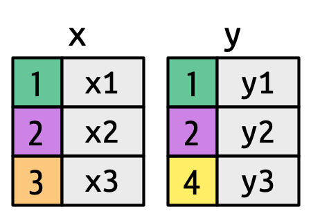
Here, we see that that these tables have some shared rows (1 and 2) but some non-shared rows (3 in table x and 4 in table y). Ultimately, different joins will differ in how they treat those non-shared rows.

To set up a join, you can conceptually think of starting with all possible pairs. For this data set, that’s \(9 = 3 \times 3\) total possible pairings:

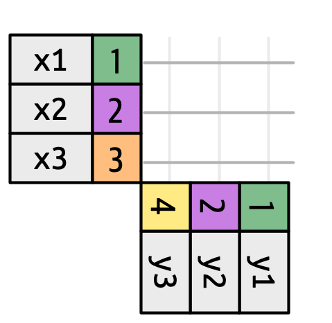
You do not generally want to actually make all these pairs when dealing with large data - this is just a mental tool.

When you add a join key (join_by()) you are specifying which of these possible pairs you are possibly interested in. All joins will capture the proper matches (1 and 2) - the only difference is in the treatment of unmatched pairs.

The most restrictive join – the inner_join – only captures true matches:

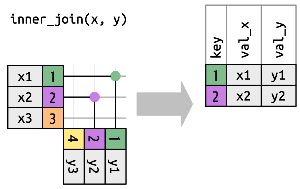
Here the green and purple (1 and 2) rows have matches so we keep them. There is no match for the orange or yellow rows so the inner_join discards them.

If we want to keep the unmatched orange 3, we might use a left_join:

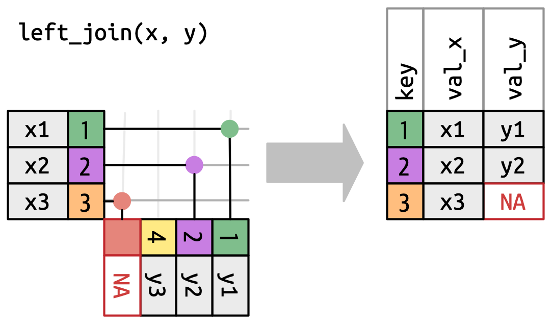
Here you’re seeing that we keep everything in the left (x table). We don’t have a matching row in the y table, but that’s ok - we just fill it in with our missing value NA.

The right_join is the exact opposite:

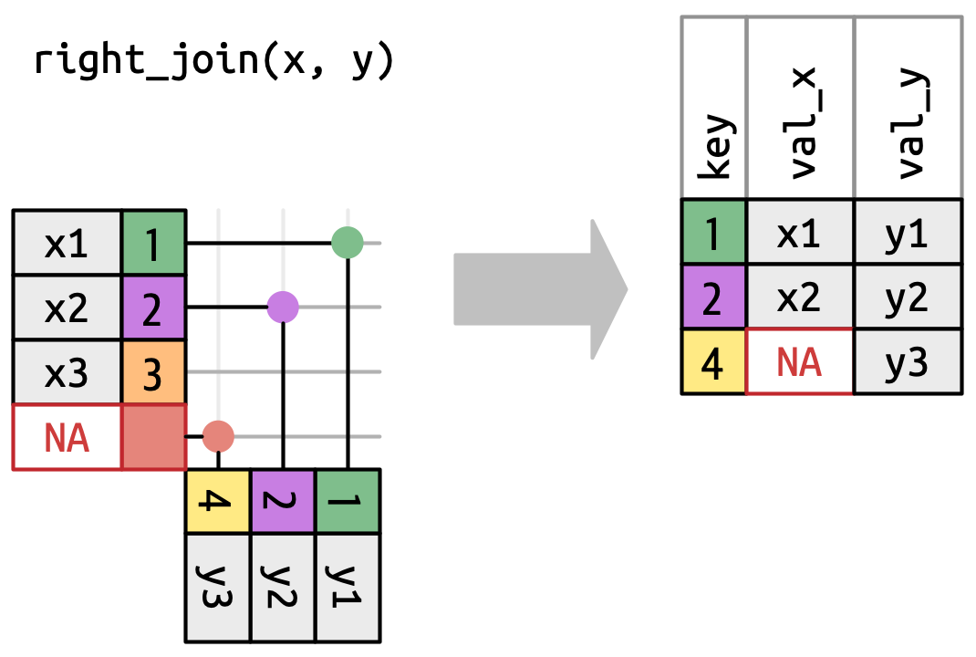
Here, we keep everything from the right / bottom / second table. Specifically, we keep the yellow 4, but discard the orange 3. As before, we fill in the missing value for the x column with an NA.

Finally, the full_join keeps everything:

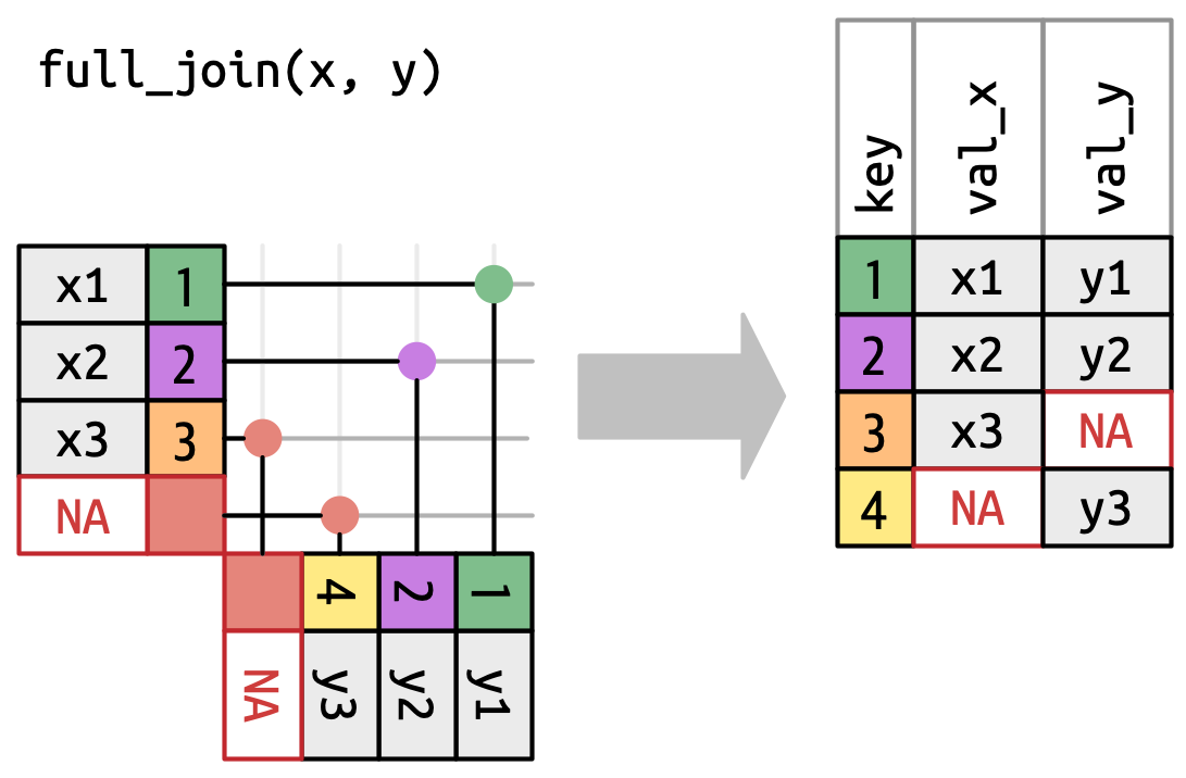Note importantly that this doesn’t force a match for orange 3 or yellow 4. They are still both unmatched, so they both wind up with NA values. Because the missing data comes from different tables, we now have an NA in both columns.

If you think this all sounds like Venn diagrams and set theory, you aren’t wrong:

At this point, you are probably asking yourself when you should use which type of join. There unfortunately isn’t a one-size fits all answer. For me, the choice of join is essentially equivalent to how you want to handle missing values.

An inner_join is essentially the same as automatically passing na.rm=TRUE to all downstream analysis, while a left_join or similar will produce NAs you have to deal with later. If the NAs are going to be relevant - e.g., if you want to report the number of unmatched values - I’d use a left_join, but otherwise I find myself reaching for inner_join by default.

It is sometimes worthwhile to abstract this a bit to think about why your data is missing: in statistics, we often think about three models of missingness:

Missing Completely at Random (MCAR)
Missing at Random (MAR)
Missing Not at Random (MNAR)

MCAR missingness - when the missingness is truly random and unrelated to any variables of interst - is a strong and rare condition, but it’s really the only situation where it’s totally safe to just drop missing values.

Dealing with missing data is a bit of an art and often easier to discuss on concrete problems than in the abstract. E.g, in our flights data, the missing values (is.na(arr_delay) == TRUE) correspond to cancelled flights. These aren’t MCAR and they are actually MNAR (the worst case): they are missing precisely because they would have been huge delays. If you simply throw them out, you are technically reporting an accurate value, but you are obscuring a deeper underlying truth.

Extra: Going Deeper with Joins

We won’t discuss them here, but there are several additional types of joins you might use on rare occasion. I wouldn’t worry about mastering them now, but for completeness:

full_join: this essentially combines the left_join and right_join and never drops rows from either table, even if unmatched
semi_join: this is essentially an inner_join(x, y) that then throws away the y columns and only keeps x. This is primarily useful when you are checking that you have data that can be properly joined later in the analysis or if you have a “gold standard” table you want to be sure you are only looking at subsets of.
anti_join: this is the opposite of an inner_join or semi_join. anti_join(x, y) returns the rows of x that don’t have a match in y. This is mainly used for finding missing data. E.g., I use an anti_join in some of my code to find students who haven’t submitted an assignment by anti-joining my list of students with the list of submissions I have received.
cross_join: the cross join is essentially the “maximal” join and it returns all possible combinations without doing any subsetting or filtering, i.e., no join_by statement. This is a bit dangerous to use on anything but small data sets since it can create many rows quickly.

You can also pass more complex operations to the join_by operator:

Inequality joins: you can do something like join_by(x >= y). This can be used to do things like cumulative operators for time series:

This is rather advanced.
In other circumstances, you won’t have exact equality to match on and can do “nearest” joins using the closest() or between() functions.

Additional `dplyr` functionality

dplyr provides some additional functionality that is often useful. While these functions are not as important as the SQL-type verbs we’ve covered above, it is worth being aware of them so that you have a starting point if these types of questions come up in your mini-projects or course project. Unlike the *_join family, there isn’t really an overarching “theory” of these functions: they are just things that come up in data analysis.

Vector Functions

Most of the functions we have discussed to this point in the course are either fully vectorized (+, cos, sqrt) or fully summarizing (length, sum, min). There is a third class of functions which are vector-in+vector-out but that also need to look at the whole vector. I divide these broadly into the three categories below.

Ranking Values

Often, you will want to put “ranks” or “orders” next to values, so that you can see what is the highest, second highest, etc. While you can get the highest or lowest values rather easily with min and max, getting other ranks is harder.

These three functions - row_number, min_rank, and dense_rank - are best illustrated by an example:

library(dplyr)
data.frame(x = c(1.5, 3, 10, 15, 10, 4)) |> 
    mutate(rn = row_number(x), 
           mn = min_rank(x), 
           dr = dense_rank(x))

     x rn mn dr
1  1.5  1  1  1
2  3.0  2  2  2
3 10.0  4  4  4
4 15.0  6  6  5
5 10.0  5  4  4
6  4.0  3  3  3

As you can see, these differ in how they handle ties (here the two x=10 rows):

row_number gives the lower rank to whichever row comes first
min_rank gives them both the lower rank and then “skips” to make up
dense_rank gives them both the lower rank, like min_rank, but doesn’t skip values to account for the tie

This brings up an important element of these types of functions: they are the first things we have seen that are sensitive to row order! This makes them a bit unpredictable so if you need tight quality control of outputs, it’s usually a good idea to have an arrange just before using them.

In more statistical contexts, we might use percentiles instead of ranks:

data.frame(x = c(1.5, 3, 10, 15, 10, 4)) |> 
    mutate(pr = percent_rank(x), 
           cd = cume_dist(x))

     x  pr        cd
1  1.5 0.0 0.1666667
2  3.0 0.2 0.3333333
3 10.0 0.6 0.8333333
4 15.0 1.0 1.0000000
5 10.0 0.6 0.8333333
6  4.0 0.4 0.5000000

Here the percentiles let us say, e.g., 60% of other rows are below this row. The methods differ essentially in how they treat the endpoints.

Cumulative (Running) Values

Particularly when dealing with temporal data, cumulative statistics may be useful:

data.frame(date = Sys.Date() - seq(7, 1), 
           value = c(1, 5, 10, 25, 50, 100, 500)) |>
    mutate(cum_mean = cummean(value), 
           cum_sum  = cumsum(value), 
           cum_max  = cummax(value), 
           cum_min  = cummin(value))

        date value  cum_mean cum_sum cum_max cum_min
1 2025-09-23     1  1.000000       1       1       1
2 2025-09-24     5  3.000000       6       5       1
3 2025-09-25    10  5.333333      16      10       1
4 2025-09-26    25 10.250000      41      25       1
5 2025-09-27    50 18.200000      91      50       1
6 2025-09-28   100 31.833333     191     100       1
7 2025-09-29   500 98.714286     691     500       1

Clearly, this sort of cumulative value is highly sensitive to row order.

It is also worth distinguishing cumulative values - which include all values up to that point - from running values - which only use a fixed lookback window. Running statistics are not included in dplyr and will require other packages.

Shift Functions

Similarly, in time series, it is useful to look at the previous or next values to compute things like percent change. Here the lead and lag functions may be helpful:

data.frame(date = Sys.Date() - seq(7, 1), 
           value = c(1, 5, 10, 25, 50, 100, 500)) |>
    mutate(prev_value = lag(value), 
           pct_change = 100 *(value / prev_value - 1))

        date value prev_value pct_change
1 2025-09-23     1         NA         NA
2 2025-09-24     5          1        400
3 2025-09-25    10          5        100
4 2025-09-26    25         10        150
5 2025-09-27    50         25        100
6 2025-09-28   100         50        100
7 2025-09-29   500        100        400

Conditional Manipulations

As we have seen, the mutate command can be used to perform a transformation to all rows. Sometimes, we only want to perform a transformation to certain rows or to perform different transformations depending on the values of one or more columns. In this context, things like if_else and case_when may be useful:

data.frame(x = c(-3, -2, -1, 0, 1, 2, 3)) |>
    mutate(x_pos_squared = if_else(x > 0, x^2, 0))

   x x_pos_squared
1 -3             0
2 -2             0
3 -1             0
4  0             0
5  1             1
6  2             4
7  3             9

Here, the if_else command checks whether the condition is true (if x is positive): if it is, we get the value of the first argument (x^2); if it is not true, we get the second (0).

The case_when operator generalizes this to 3 or more cases:

data.frame(x = c(-3, -2, -1, 0, 1, 2, 3), 
           group=c("cos", "sin", "tan", "cos", "sin", "sin", "tan")) |>
    mutate(x_trig = case_when(
        group == "cos" ~ cos(x), 
        group == "sin" ~ sin(x), 
        group == "tan" ~ tan(x)
    ))

   x group     x_trig
1 -3   cos -0.9899925
2 -2   sin -0.9092974
3 -1   tan -1.5574077
4  0   cos  1.0000000
5  1   sin  0.8414710
6  2   sin  0.9092974
7  3   tan -0.1425465

Here, the case_when checks the conditions in order to figure out which transformation to apply. The syntax is a bit funny: the expression to the left of the ~ is the thing checked to see if it is true; the value on the right of the ~ is the value returned. Because of this, you can set defaults by putting a TRUE ~ in the final case:

data.frame(x = c(-3, -2, -1, 0, 1, 2, 3), 
           group=c("cos", "sin", "unknown", "cos", "sin", "sin", "unknown")) |>
    mutate(x_trig = case_when(
        group == "cos" ~ cos(x), 
        group == "sin" ~ sin(x), 
        TRUE  ~ NA
    ))

   x   group     x_trig
1 -3     cos -0.9899925
2 -2     sin -0.9092974
3 -1 unknown         NA
4  0     cos  1.0000000
5  1     sin  0.8414710
6  2     sin  0.9092974
7  3 unknown         NA

Note that this is all still evaluated row-by-row independently. If you want to do groupwise operations, you need a group_by and likely a summarize to follow.

penguins |>
    group_by(species) |>
    mutate(label = case_when(
        body_mass == max(body_mass, na.rm=TRUE) ~ "Biggest of Species", 
        body_mass == min(body_mass, na.rm=TRUE) ~ "Smallest of Species", 
        TRUE ~ "In the middle"
    ))

# A tibble: 344 × 9
# Groups:   species [3]
   species island    bill_len bill_dep flipper_len body_mass sex     year label 
   <fct>   <fct>        <dbl>    <dbl>       <int>     <int> <fct>  <int> <chr> 
 1 Adelie  Torgersen     39.1     18.7         181      3750 male    2007 In th…
 2 Adelie  Torgersen     39.5     17.4         186      3800 female  2007 In th…
 3 Adelie  Torgersen     40.3     18           195      3250 female  2007 In th…
 4 Adelie  Torgersen     NA       NA            NA        NA <NA>    2007 In th…
 5 Adelie  Torgersen     36.7     19.3         193      3450 female  2007 In th…
 6 Adelie  Torgersen     39.3     20.6         190      3650 male    2007 In th…
 7 Adelie  Torgersen     38.9     17.8         181      3625 female  2007 In th…
 8 Adelie  Torgersen     39.2     19.6         195      4675 male    2007 In th…
 9 Adelie  Torgersen     34.1     18.1         193      3475 <NA>    2007 In th…
10 Adelie  Torgersen     42       20.2         190      4250 <NA>    2007 In th…
# ℹ 334 more rows

Here, as always, the min and max are computed groupwise, i.e., per species, because of the group_by that comes before.

Extra: Multi-Column Operations

We sometimes do need to put multiple columns together, e.g., to get the student’s highest score on three attempts at a test. This can be done with the c_across operator, but I honestly find it a bit confusing and prefer to do some pivot magic:

student_grades <- tribble(
    ~name,    ~test1, ~test2, ~test3, 
    "Alice",      90,     80,    100,
    "Bob",        90,     90,     80,
    "Carol",      50,    100,    100,
    "Dave",      100,      0,      0)

student_grades |> 
    rowwise() |> # Make each row its own group so that we don't accidentally combine
    mutate(max_test = max(c_across(c(test1, test2, test3))), 
           avg_test = mean(c_across(c(test1, test2, test3))))

# A tibble: 4 × 6
# Rowwise: 
  name  test1 test2 test3 max_test avg_test
  <chr> <dbl> <dbl> <dbl>    <dbl>    <dbl>
1 Alice    90    80   100      100     90  
2 Bob      90    90    80       90     86.7
3 Carol    50   100   100      100     83.3
4 Dave    100     0     0      100     33.3

This is pretty fragile and a bit slow due to the rowwise() operator which makes every row its own groups, so I personally find the pivot approach easier for this:

library(tidyr) # For pivot_longer
student_grades |>
    pivot_longer(cols=c(test1, test2, test3), 
                 names_to="test", 
                 values_to="score") |>
    group_by(name) |>
    summarize(max_test = max(score), 
              avg_test = mean(score))

# A tibble: 4 × 3
  name  max_test avg_test
  <chr>    <dbl>    <dbl>
1 Alice      100     90  
2 Bob         90     86.7
3 Carol      100     83.3
4 Dave       100     33.3

But chacun à son goût.

Exercises

Answer the following questions using the various techniques described above.

Identify the top 5 days by largest fraction of flights delayed.
Solution
Note a few points of danger to be aware of here:
1. dense_rank and company sort in ascending order, so we need to use the desc modifier to reverse the rankings.
2. You have to ungroup after summarize or you will do rankings within each group (here, month), which gives incorrect values.
If you want to modify your code to make the result a bit more attractive, this snippet has some useful tricks:
Create a table of the daily YTD mean average departure delay for all flights departing Newark airport.

Hint: You can first group by days and compute daily averages, then compute the YTD quantities or you can compute a cumulative statistic over all flights and then take end of day values using last(). These are slightly different, but should not differ greatly, as they essentially just vary in whether days are weighted by number of flights.

Solution

First approach:

Second approach:
Which day had the largest increase in number of delayed flights over the previous day?

Solution
To this point, we have looked at average delay using both the positive and negative values in that column. This gives airlines ‘credit’ for flights that leave early, but may understate the true delays experienced by passengers. Create a new column measuring real delays by setting negative delays (early departures) to zero and compute the average delay per airline.

Solution
Using your average real delay statistics, which airline has the largest difference in average delay with and without credit for early departures.

Solution

I have included a few extra steps to optimize formatting near the end.

Footnotes

Note that some SQL engines use LEFT OUTER JOIN than LEFT JOIN. Because OUTER is a bit ambiguous, dplyr emphasizes full_ vs left_ in its function naming. Also note the convention of dplyr names - lower case, underscore separated - and that it differs from SQL syntax.↩︎

Slides

Review Practice

Multi Table Operations

Join Specifications

Inner Joins

Left Join

Selecting Join Types

Additional dplyr functionality

Vector Functions

Ranking Values

Cumulative (Running) Values

Shift Functions

Conditional Manipulations

Exercises

Footnotes

Additional `dplyr` functionality